S2: Linear Combinations of Random Variables
The Ultimate Mashup: Combining Random Variables 🔀
Introduction
1. Introduction
Hey there! Ever wondered what happens when you mix different random events together? Like, what's the average total weight of groceries in two shopping bags, or the difference in scores between two friends in a game? That's exactly what we're diving into in this chapter! We'll start by figuring out the new mean (expectation) and variance when we add, subtract, or scale random variables. Then, we'll uncover a super important rule about how variance behaves when we combine independent variables (spoiler: it's a bit unexpected!). Finally, we'll see how the awesome properties of the Normal distribution make combining Normal variables incredibly straightforward. Get ready to level up your stats game! 🚀
2. Expectation and Variance of Linear Transformations
Alright, let's talk about transforming our random variables. Think of it like putting a filter on a Snapchat pic, you're taking the original data and changing it in a consistent way. In math, we call this a linear combination, which looks like . Here, is our original random variable (like the number of hours you work), and is the new, transformed variable (like your weekly pay).
The 'b' part is a shift. It's like adding 5 points to everyone's test score because the first question was unfair. The whole dataset just slides up or down the number line. This changes the average, of course, but does it change how spread out the scores are? Nope! The gap between the top score and the bottom score is still the same. That's the key intuition here.
The 'a' part is a scaling. This is like your boss deciding to double your hourly wage (we wish!). This stretches or squishes your data. It definitely changes the average, but it also changes the spread. If your hours vary, doubling the pay rate will make the difference between a good week's pay and a bad week's pay much larger.
The 'b' part is a shift. It's like adding 5 points to everyone's test score because the first question was unfair. The whole dataset just slides up or down the number line. This changes the average, of course, but does it change how spread out the scores are? Nope! The gap between the top score and the bottom score is still the same. That's the key intuition here.
The 'a' part is a scaling. This is like your boss deciding to double your hourly wage (we wish!). This stretches or squishes your data. It definitely changes the average, but it also changes the spread. If your hours vary, doubling the pay rate will make the difference between a good week's pay and a bad week's pay much larger.
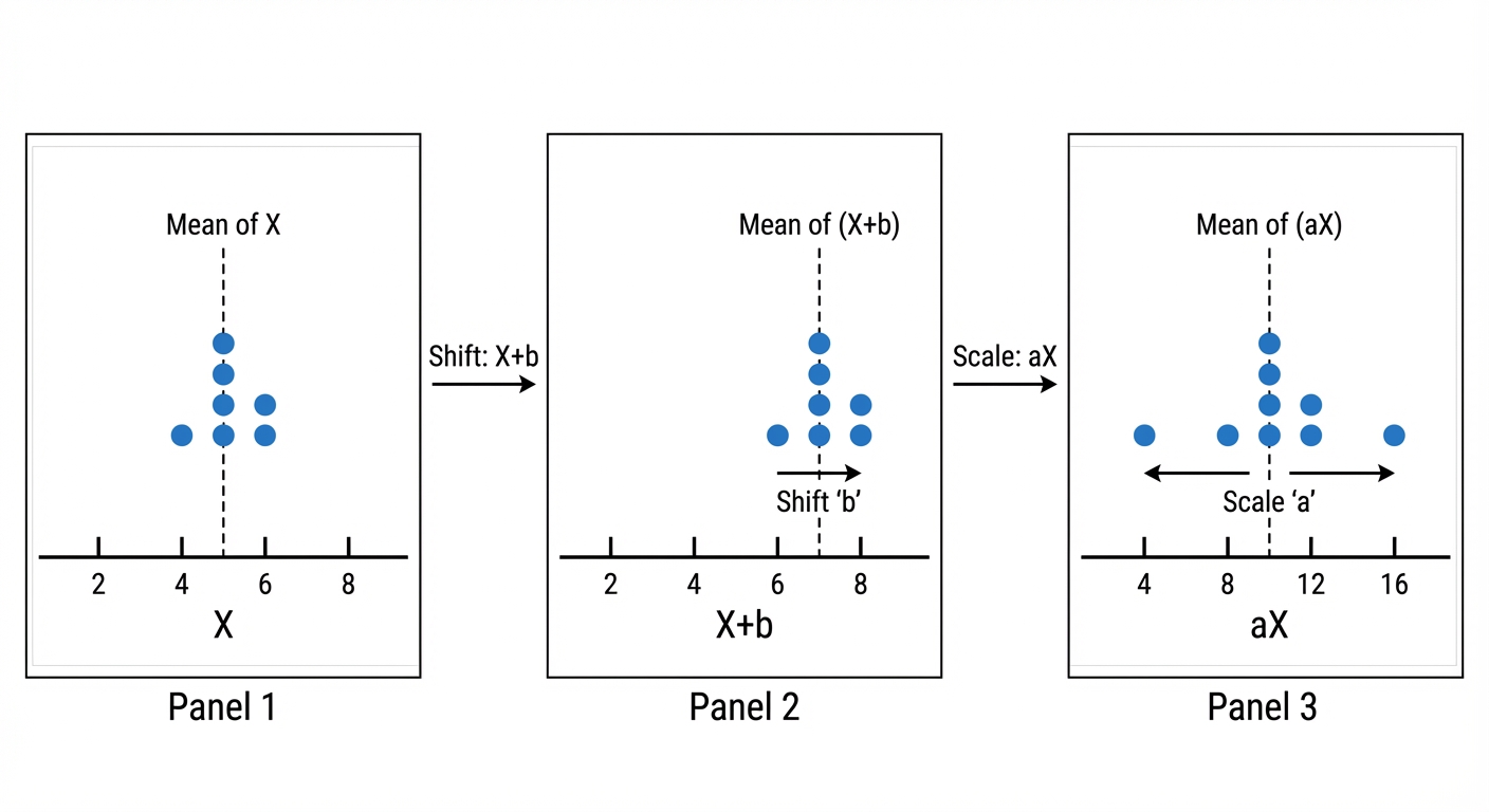
So, how does this affect our stats? The rules are super slick:
1. Expectation (The Mean): . This makes perfect sense. The average value gets scaled by 'a' AND shifted by 'b'. It's affected by both moves.
2. Variance (The Spread): . Notice anything missing? The 'b' is gone! The shift doesn't affect the spread, so we ignore it. The scaling factor 'a' is squared because variance is measured in squared units. Remember, standard deviation is the square root of variance, so . When you square that to get back to variance, you get . Easy peasy!
Worked example
Worked Example: Calculating Weekly Earnings
From Hours Worked to Actual Cash 🤑
The number of hours, , a student works per week at a streaming service's call centre is a random variable with an expectation and a variance . The student earns £11 per hour but has fixed weekly travel costs of £15. Let be the student's weekly profit. Find the expectation and variance of .
- 1First, let's identify the information we're given for our original random variable, (the hours worked).
- 2Now, we need to set up the linear equation for the weekly profit, . The student earns £11 for every hour () and then has a fixed cost of £15 (). This gives us the form .
- 3Let's find the expected profit, , using the rule . We'll plug in our values for , , and .
- 4Next, we'll find the variance of the profit, , using the rule . Remember, the shift (travel cost) doesn't affect the spread of the earnings!
- 5Finally, let's state our answers clearly with the correct units. Expectation is in pounds, and variance is in pounds squared.
Answer
3. Variance of Linear Combinations of Independent Random Variables
Alright, let's level up. You know what random variables are, things with unpredictable outcomes, like the number of likes on your next Insta post () or how many minutes you spend watching TikToks before starting homework (). The key word for this concept is independent. This just means the outcome of has zero effect on the outcome of . Your Insta likes don't change your TikTok habits. They're in their own lanes, unbothered.
Now, what happens when we combine them? Let's say we have a new variable, . The big rule you need to lock in is: This formula is your new best friend. Notice two epic things: First, the constants and get squared. This is because variance is measured in squared units (like ), so any scaling factor has to be squared to match. Second, and this is the part that trips everyone up, we always add the resulting variances.
Now, what happens when we combine them? Let's say we have a new variable, . The big rule you need to lock in is: This formula is your new best friend. Notice two epic things: First, the constants and get squared. This is because variance is measured in squared units (like ), so any scaling factor has to be squared to match. Second, and this is the part that trips everyone up, we always add the resulting variances.
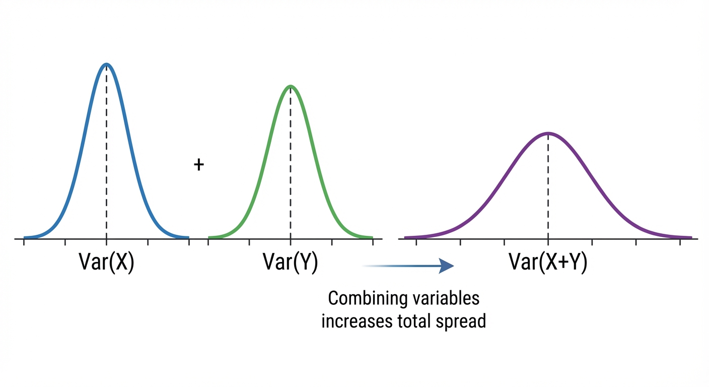
Even if you're calculating the variance of a difference, like , the formula is still . Why? Because variance is a measure of unpredictability or 'spread'. Whether you add two unpredictable things or find the difference between them, the total potential for variation only goes up. The chaos just stacks! So remember: square the constants, and always, always add the variances.
Several separate items vs one item multiplied. This is the classic trap. If you add independent observations of (three separate smoothies, five separate bags), write : then but If instead one observation is multiplied by (one bag's weight tripled, ), then . The means agree ( either way), but the variances do not. Read the question: "3 separate items" means , not .
Several separate items vs one item multiplied. This is the classic trap. If you add independent observations of (three separate smoothies, five separate bags), write : then but If instead one observation is multiplied by (one bag's weight tripled, ), then . The means agree ( either way), but the variances do not. Read the question: "3 separate items" means , not .
Worked example
Worked Example: Calculating Variance and Standard Deviation
The Smoothie Shack Scenario 🥤
You work at a smoothie shack. The volume of juice in a 'Regular' smoothie, , is a random variable with a standard deviation of 4 ml. The volume of juice in a 'Jumbo' smoothie, , is a random variable with a standard deviation of 6 ml. The volumes are independent.
A customer orders 3 Regular smoothies and 2 Jumbo smoothies. Find the standard deviation of the total volume of juice required.
A customer orders 3 Regular smoothies and 2 Jumbo smoothies. Find the standard deviation of the total volume of juice required.
- 1First up, we need to find the variance for each smoothie type. Remember, variance is just the standard deviation squared (). We're given the standard deviations, so let's convert them.
- 2Next, let's define our new random variable for the total volume, . The customer wants 3 separate Regulars and 2 separate Jumbos. Each smoothie varies independently, so this is a sum of five independent volumes, not (that would mean one Regular smoothie's volume tripled).
- 3Now we add the variances, one for each smoothie. For a sum of independent copies, the variance is , not .
- 4Let's plug in the variance values we calculated in Step 1 and solve for .
- 5The question asks for the standard deviation of the total volume, not the variance. So, the final step is to take the square root. (Writing would give and an SD of , which is wrong for this situation.)
Answer
4. The Distribution of Linear Combinations of Normal Variables
Alright, let's talk about the ultimate team-up in stats: combining normal distributions. Think of it like a collab between your two favorite artists, when they get together, you get a whole new track that's still awesome. The big rule here is: if you take two independent normal random variables, let's call them and , and you mix them together in a linear combination like , the result is also a normal distribution. It's like a superpower of the normal distribution! The 'independent' part is key, it means what happens with has zero effect on what happens with , like your gaming K/D ratio is independent of your friend's Snapchat story views.
So, if we have and , how do we figure out the new distribution for a variable like ? We just need its mean and variance.
1. The New Mean: The mean of the combination is just the combination of the means. Super intuitive. 2. The New Variance: This is where you gotta be careful. The variance of the combination is Notice how the constants and get squared! Also, a massive trap alert 🚨: variances always add for independent variables, even if you're subtracting (like for , the variance would be ). Uncertainty always piles up!
So, if we have and , how do we figure out the new distribution for a variable like ? We just need its mean and variance.
1. The New Mean: The mean of the combination is just the combination of the means. Super intuitive. 2. The New Variance: This is where you gotta be careful. The variance of the combination is Notice how the constants and get squared! Also, a massive trap alert 🚨: variances always add for independent variables, even if you're subtracting (like for , the variance would be ). Uncertainty always piles up!
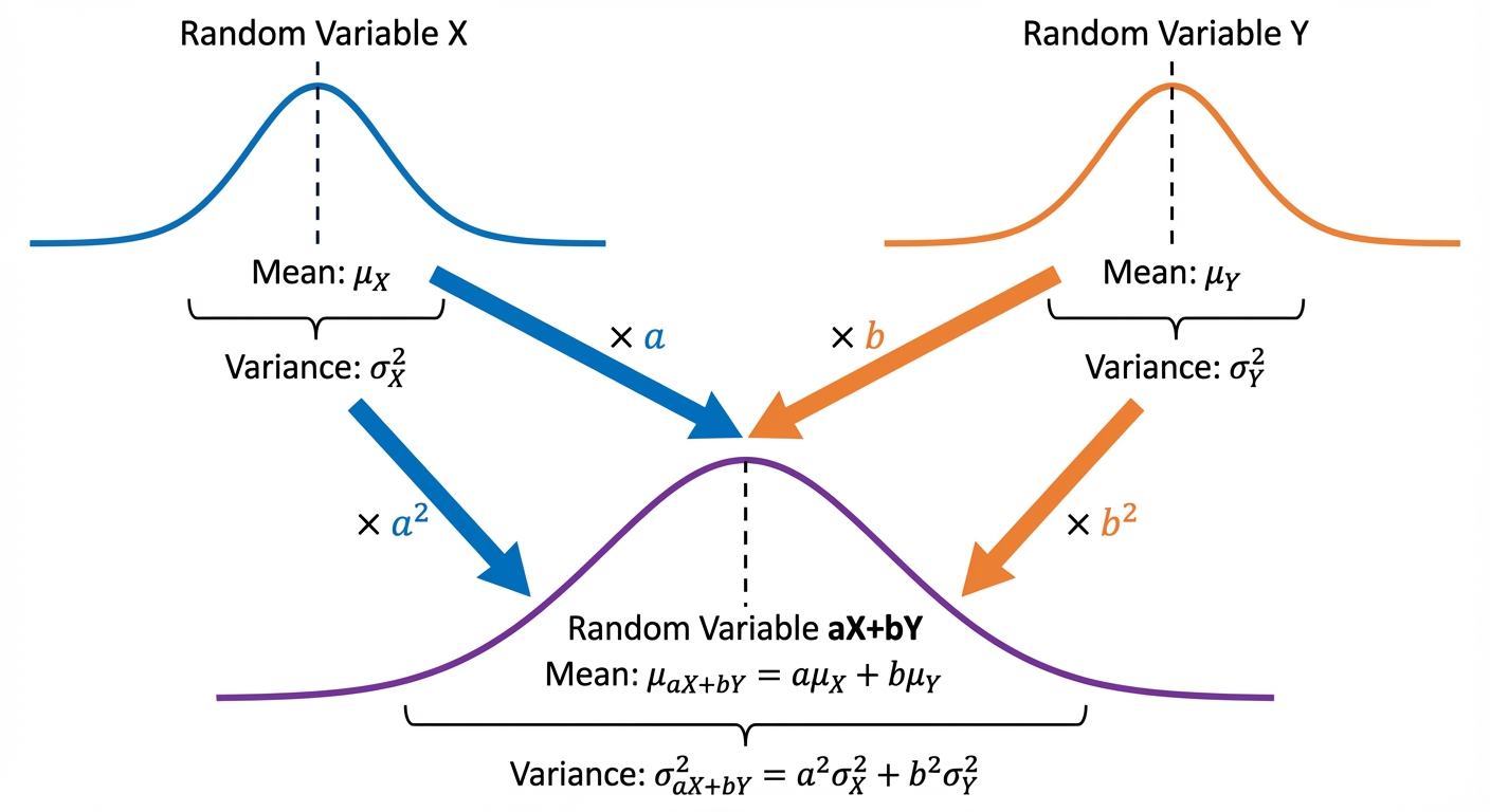
So, the final distribution is just . Once you have this new normal distribution, you can solve problems just like you always do, by standardizing to find a Z-score and looking up the probability. You got this!
Worked example
Worked Example: Probability of a Sum of Normal Variables
Worked Example: The Part-Time Job Paycheck Problem 💰
You work two part-time jobs. Your weekly pay from your cafe job, , is normally distributed with a mean of £80 and a standard deviation of £10. Your pay from your weekend tutoring job, , is independently normally distributed with a mean of £50 and a standard deviation of £8. What is the probability that your total pay in one week is more than £140?
- 1First, let's define a new variable for the total pay, . Since and are independent normal variables, our total pay will also be normally distributed. Our mission is to find the mean and variance of .
- 2Let's find the mean of our total pay, . This is straightforward, we just add the individual means together.
- 3Now for the variance, . This is the tricky part! Remember to use variances (standard deviation squared), and for independent variables, variances always add.
- 4Awesome, we've got the mean and variance for our total pay. We can now state its full distribution.
- 5Finally, we can solve the problem. We need to find . We'll standardize this to a Z-score and then use our calculator or tables to find the probability.
Answer
Practice this in the app
Unlock the full chapter: practice questions, flashcards, mock papers and notes, free.
Continue revising