S2: Continuous Random Variables
When Random Gets Smooth 📈
Introduction
1. Introduction
Hey there! So far in statistics, we've mostly dealt with discrete random variables—things you can count, like the number of heads in a coin toss. But what about things you measure? Think height, weight, or the time it takes to run a race. These can take on any value in a range, and that's where Continuous Random Variables come in. It's a whole new ball game! 🤩
In this chapter, we're going to dive into the world of smooth, continuous data. First, we'll meet the Probability Density Function (PDF), which is like the rulebook for a continuous variable. Then, we'll learn how to calculate the mean and variance using our old friend, integration. Finally, we'll put it all together to find probabilities and percentiles, answering questions like 'What's the chance the bus arrives in the next 5 minutes?' It might sound tricky, but it's just about seeing probability as an area under a curve. Let's get started!
In this chapter, we're going to dive into the world of smooth, continuous data. First, we'll meet the Probability Density Function (PDF), which is like the rulebook for a continuous variable. Then, we'll learn how to calculate the mean and variance using our old friend, integration. Finally, we'll put it all together to find probabilities and percentiles, answering questions like 'What's the chance the bus arrives in the next 5 minutes?' It might sound tricky, but it's just about seeing probability as an area under a curve. Let's get started!
2. Properties of Probability Density Functions
Alright, let's dive into Probability Density Functions, or PDFs. In S1, we dealt with discrete random variables – like the number you get when you roll a die (you can get a 2 or a 3, but not 2.5). Now in S2, we're levelling up to continuous random variables, which can take any value in a range. Think about the exact time you wait for your food delivery, the length of your favourite song, or the precise height of a person. It's not just whole numbers; it's decimals galore.
A PDF, written as , is basically a curve that models the probability distribution for these continuous variables. It has two golden rules you absolutely have to know. They're like the non-negotiable terms and conditions of the math world.
First, for all . This just means the graph of the PDF never dips below the x-axis. It makes perfect sense, right? Probability can't be negative. You can't have a -20% chance of your crush texting you back. It's either 0% or higher. Simple.
Second, and this is the big one, the total area under the curve is always equal to 1. In calculus terms, that's . This is like saying the probability of something happening is 100%. The chance that your bus arrives at some point in time is 1. The chance that your gaming PC's temperature is some value within its operating range is 1.
A PDF, written as , is basically a curve that models the probability distribution for these continuous variables. It has two golden rules you absolutely have to know. They're like the non-negotiable terms and conditions of the math world.
First, for all . This just means the graph of the PDF never dips below the x-axis. It makes perfect sense, right? Probability can't be negative. You can't have a -20% chance of your crush texting you back. It's either 0% or higher. Simple.
Second, and this is the big one, the total area under the curve is always equal to 1. In calculus terms, that's . This is like saying the probability of something happening is 100%. The chance that your bus arrives at some point in time is 1. The chance that your gaming PC's temperature is some value within its operating range is 1.
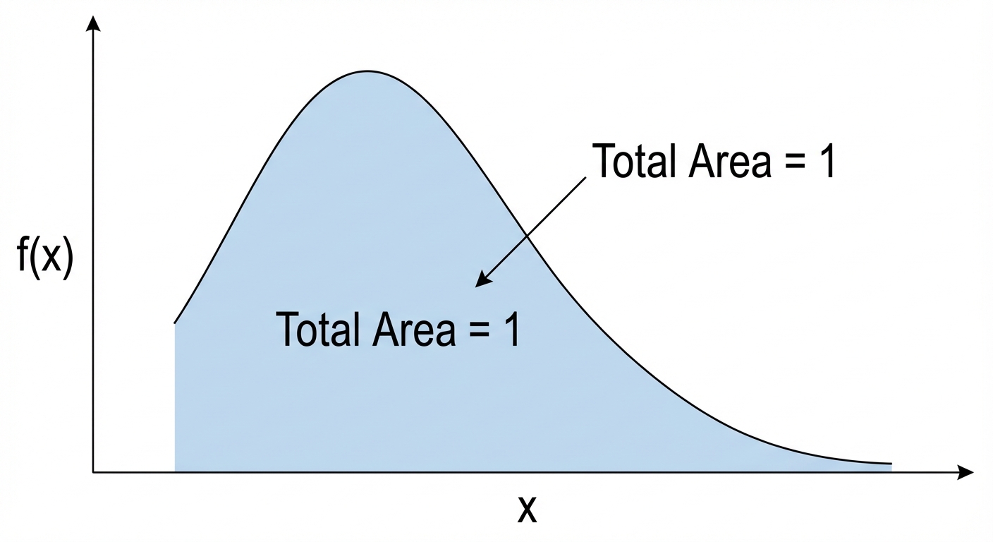
. This rule is super important because it allows us to find unknown constants in the function, often called 'k', by setting up an integral and making it equal to 1. We call this finding the 'normalising constant'.
Worked example
Worked Example: Finding the Normalising Constant
Solving for 'k' - The Unlockable Character 🔓
The continuous random variable has a probability density function given by:
Find the value of the constant .
Find the value of the constant .
- 1Okay, first things first. We know that for any PDF, the total area under the curve must equal 1. This is our non-negotiable starting point. We'll set up a definite integral for our function over its given domain and set it equal to 1.
- 2Now, let's substitute our function into the integral. The domain for our function is from to . Everywhere else it's zero, so we don't need to worry about other intervals.
- 3Time for some calculus! Since is just a constant, we can pull it outside the integral to make life easier. Then we integrate the function with respect to .
- 4Next, we evaluate the integral by plugging in the limits. We substitute the upper limit (2) and subtract what we get when we substitute the lower limit (0).
- 5Let's simplify that expression. The second bracket is just zero, which is nice. Now we just have a simple equation to solve for our mystery constant, .
- 6And for the final move! Just a little bit of algebraic rearranging to isolate . And boom, we've found our normalising constant. GG! ✨
Answer
3. Probability and Percentiles from a PDF
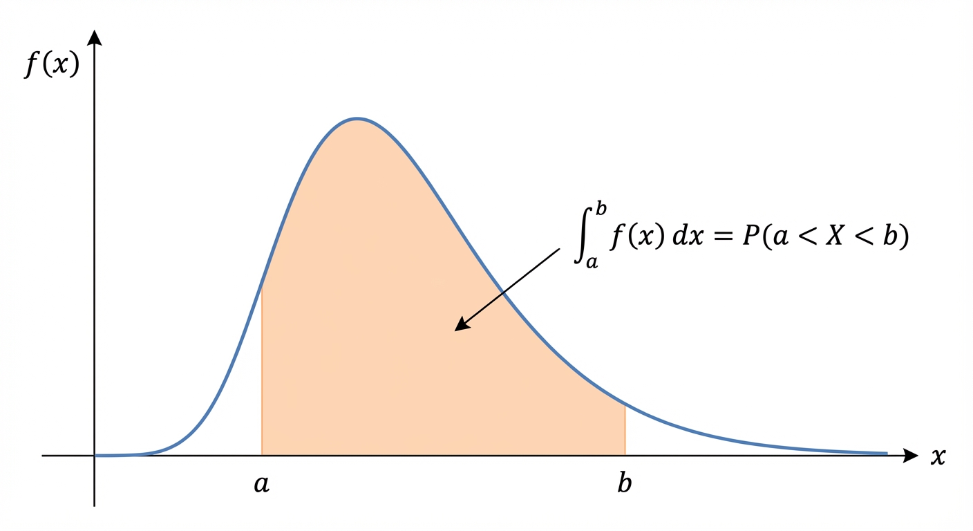
Alright, let's get into it. With continuous random variables, the probability of being exactly one specific value is zero. Think about it: what are the odds your bus arrives at precisely 8:15:00.000... AM? Infinitesimally small! Instead, we care about the probability that falls within a range, like your bus arriving between 8:15 and 8:20. To find this probability, , we find the area under the Probability Density Function (PDF) graph between points and . And how do we find the area under a curve? You guessed it – integration! It's the ultimate tool for this job. You simply calculate the definite integral of the PDF, , from to : .
Now, let's talk about medians and percentiles. The median () is just the 50th percentile – it's the value that splits the entire probability distribution right down the middle. 50% of the data is below it, 50% is above it. It's like finding the exact halfway point in a gaming level. To find it, we set up an integral from the lowest possible value of (let's call it ) up to the median, , and set the total probability (the area) equal to 0.5. So, we solve the equation: . This same logic applies to any percentile! If you want to find the 80th percentile (the value that 80% of the data is below), you just set the integral equal to 0.80. For the percentile, you solve for in . It's a super powerful way to understand the spread and key points of your data.
Worked example
Worked Example: Delivery Time Analysis
When is my pizza getting here?! 🍕
The waiting time, minutes, for a food delivery has a probability density function given by for , and otherwise.
a) Find the probability that the waiting time is between 5 and 7 minutes.
b) Find the median waiting time.
a) Find the probability that the waiting time is between 5 and 7 minutes.
b) Find the median waiting time.
- 1For part (a), we need to find . This means we need to integrate the PDF, , from the lower limit of 5 to the upper limit of 7. This integral represents the area under the curve between these two points.
- 2Now, let's solve the integral. We can take the constant outside. The integral of is . Then we evaluate this at the limits 7 and 5.
- 3For part (b), we need to find the median time, . The median is the value where the cumulative probability is 0.5. So, we'll set up an integral from the start of the domain (which is ) up to , and set it equal to 0.5.
- 4Let's solve this integral equation for . We perform the same integration as before, but with as the upper limit. This will give us an equation in terms of .
- 5Now, substitute the limits and simplify. This will lead to a quadratic equation. We'll solve it and choose the value of that actually lies within our domain of .
- 6We get two possible solutions for : and . Since the time must be between 2 and 10, we discard the negative solution. So, the median waiting time is 7.66 minutes.
Answer
4. Mean and Variance of a Continuous Random Variable
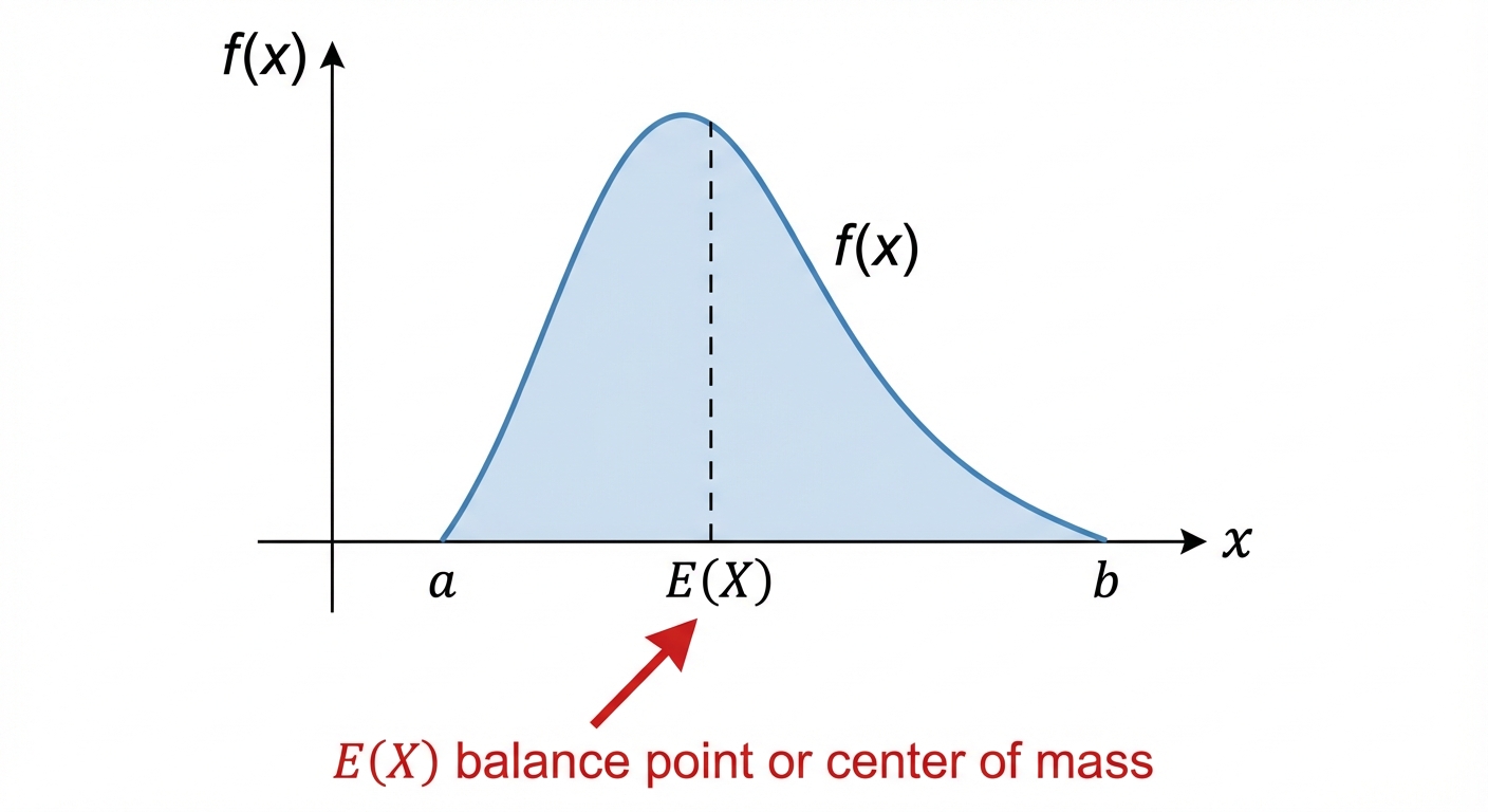
Alright, let's get into the mean and variance for continuous random variables. Think of the mean, or Expected Value , as the ultimate average. If you recorded a random variable (like the time it takes you to beat a certain game level) an infinite number of times, is the average you'd expect to get. It’s like your long-term K/D ratio. For discrete data, you'd multiply each outcome by its probability and add them up. Since we're continuous now (like a smooth audio waveform, not choppy samples), we swap the summation for an integral. The formula is your new best friend: Basically, we're integrating the value multiplied by its 'probability density' over its entire possible range.
Now, what about variance, ? Variance is all about the spread or consistency. Is your part-time job shift length super predictable (low variance) or does it change wildly week-to-week (high variance)? A low variance is like your ping in a game being super stable; high variance is major lag spikes. The formula looks a bit intense, but it's a breeze once you break it down: Let's decode this. The first part, , is just the 'mean of the squares', which we call . The second part is just the mean, , squared. So, the mantra to remember is: Variance equals the mean of the squares minus the square of the mean. You calculate first, then you calculate using a very similar integral, and finally, you plug them into the simple formula: . Easy peasy. You've got this!
Worked example
Worked Example: Mean and Variance from a PDF
Let's Get This Bread: A Part-Time Job Problem 🍞
The time, hours, that a student spends on their part-time job on a Saturday can be modelled by a continuous random variable with the probability density function for , and otherwise. Find the mean and variance of the time spent working.
- 1First up, let's find the mean, . We need to calculate the integral of between the given limits of 0 and 4. Let's expand the expression inside the integral first to make it easier to handle.
- 2Now we just do the integration, applying the power rule. Then we'll substitute the limits (4 and 0) to get our final value for the mean.
- 3Great, the mean is 2 hours. Now for the variance. First, we need the 'mean of the squares', . The setup is almost identical, but we integrate instead.
- 4Time to integrate this new expression and substitute the limits, just like we did for the mean.
- 5We have all the pieces! Now we use the magic formula: . We just plug in the values we found in steps 2 and 4.
Answer
Practice this in the app
Unlock the full chapter: practice questions, flashcards, mock papers and notes, free.
Continue revising