P1 Trigonometry: Graphs, Identities, and Equations
Trig: More Than Just SOH CAH TOA 😎
Introduction
1. Introduction
Alright, let's dive into Trigonometry! You've probably met sin, cos, and tan before, but at A-Level, we take it to a whole new level. We're going to start by visualizing these functions as graphs, understanding their wave-like patterns and how to transform them. Then, we'll ditch the calculator and master the exact trigonometric values for key angles – super useful for cleaner, more professional solutions. After that, we'll become mathematical detectives, proving trigonometric identities which are the fundamental rules that govern these functions. Finally, we'll put it all together to solve complex trigonometric equations, a skill that's a massive part of your P1 exam. It might seem like a lot, but we'll break it down step-by-step. Let's get started!
2. Derivation and Application of Exact Trigonometric Values
Alright, let's talk about one of the most clutch skills for your P1 exam: exact trigonometric values. Why are they so important? Two big reasons: non-calculator papers and future-proofing your maths brain for university. In fields like engineering or theoretical physics, 'approximately 0.866' just doesn't cut it; you need the pure, unadulterated precision of . Think of it like the difference between streaming a song in low quality vs. hearing it on lossless vinyl – one is an approximation, the other is the real deal.
So, where do these magical values come from? Not from thin air, but from two super-special triangles that you need to know like the back of your hand. Seriously, you should be able to sketch these from memory in your sleep.
First up, the 45-45-90 triangle. This is your basic isosceles right-angled triangle. Let's make the two equal sides length 1. Using Pythagoras' theorem (), the hypotenuse is .
So, where do these magical values come from? Not from thin air, but from two super-special triangles that you need to know like the back of your hand. Seriously, you should be able to sketch these from memory in your sleep.
First up, the 45-45-90 triangle. This is your basic isosceles right-angled triangle. Let's make the two equal sides length 1. Using Pythagoras' theorem (), the hypotenuse is .
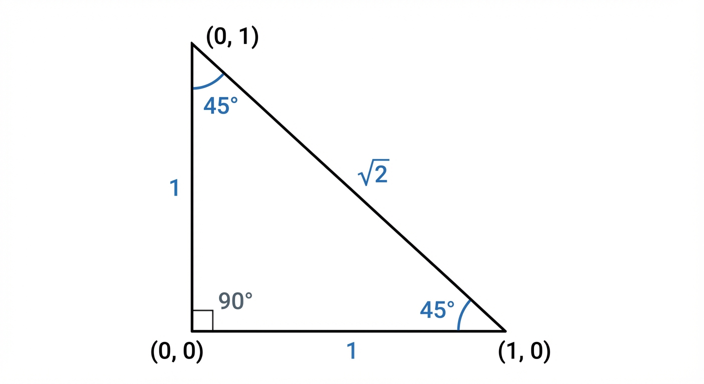
From this, we can instantly read off the values using SOH CAH TOA: , , and . Easy, right?
Next, the 30-60-90 triangle. This one is a bit more clever. Imagine an equilateral triangle with side lengths of 2. All angles are 60°. Now, drop a perpendicular line from the top vertex to the base. You've just sliced it into two identical 30-60-90 triangles!
Next, the 30-60-90 triangle. This one is a bit more clever. Imagine an equilateral triangle with side lengths of 2. All angles are 60°. Now, drop a perpendicular line from the top vertex to the base. You've just sliced it into two identical 30-60-90 triangles!
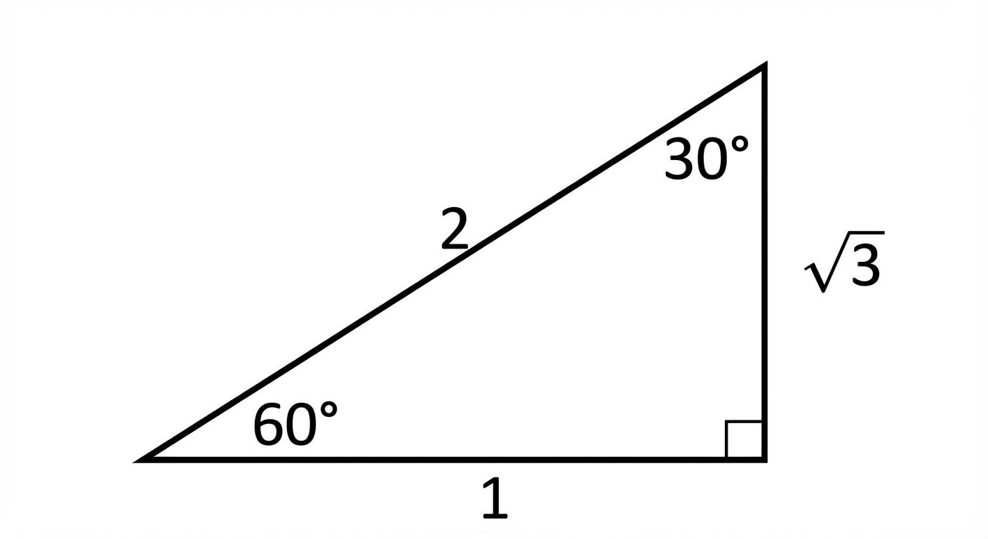
The hypotenuse is still 2, the base is now 1 (half of the original base), and the height (using Pythagoras again) is . From this single triangle, we get all the values for 30° and 60°: , , , and for 30°, , , . Memorise these triangles, not the values. It's way more efficient and less prone to error under exam pressure. These values are your building blocks for solving for related angles in other quadrants, like (which is ) or (which is ), using the CAST diagram.
Worked example
Worked Example: Evaluating an Expression with Exact Values
Worked Example: Let's Solve This Thing! 🚀
Without using a calculator, find the exact value of .
- 1First things first, let's recall the required values from our special triangles. It's like grabbing the right ingredients before you start cooking. We need: , , and .
- 2Now, let's substitute these exact values back into the original expression. This is a simple plug-and-play step, but double-check you put everything in the right place!
- 3Time to simplify. Let's tackle the multiplication first, following BIDMAS/BODMAS. Remember that multiplying a square root by itself just removes the root.
- 4Next, we evaluate the squared term. This one is pretty straightforward, but don't get complacent!
- 5Finally, let's put it all together. We just need to add the two parts. This requires finding a common denominator – a skill from way back that's still super relevant.
Answer
3. Fundamental Trigonometric Identities
Alright, let's talk about the two most important relationships in your entire trigonometric journey. Think of them less as formulas and more as fundamental truths that are always valid for any angle . These are your ultimate tools for simplifying complex expressions and proving identities, skills that are absolutely crucial for your P1 exam and for future studies in physics, engineering, or computer graphics.
First up, the big one: the Pythagorean Identity, . The '' symbol means it's an identity, true for all values of , not just an equation to be solved. Where does it come from? Imagine a point on the unit circle (a circle with radius 1). The x-coordinate is and the y-coordinate is .
First up, the big one: the Pythagorean Identity, . The '' symbol means it's an identity, true for all values of , not just an equation to be solved. Where does it come from? Imagine a point on the unit circle (a circle with radius 1). The x-coordinate is and the y-coordinate is .
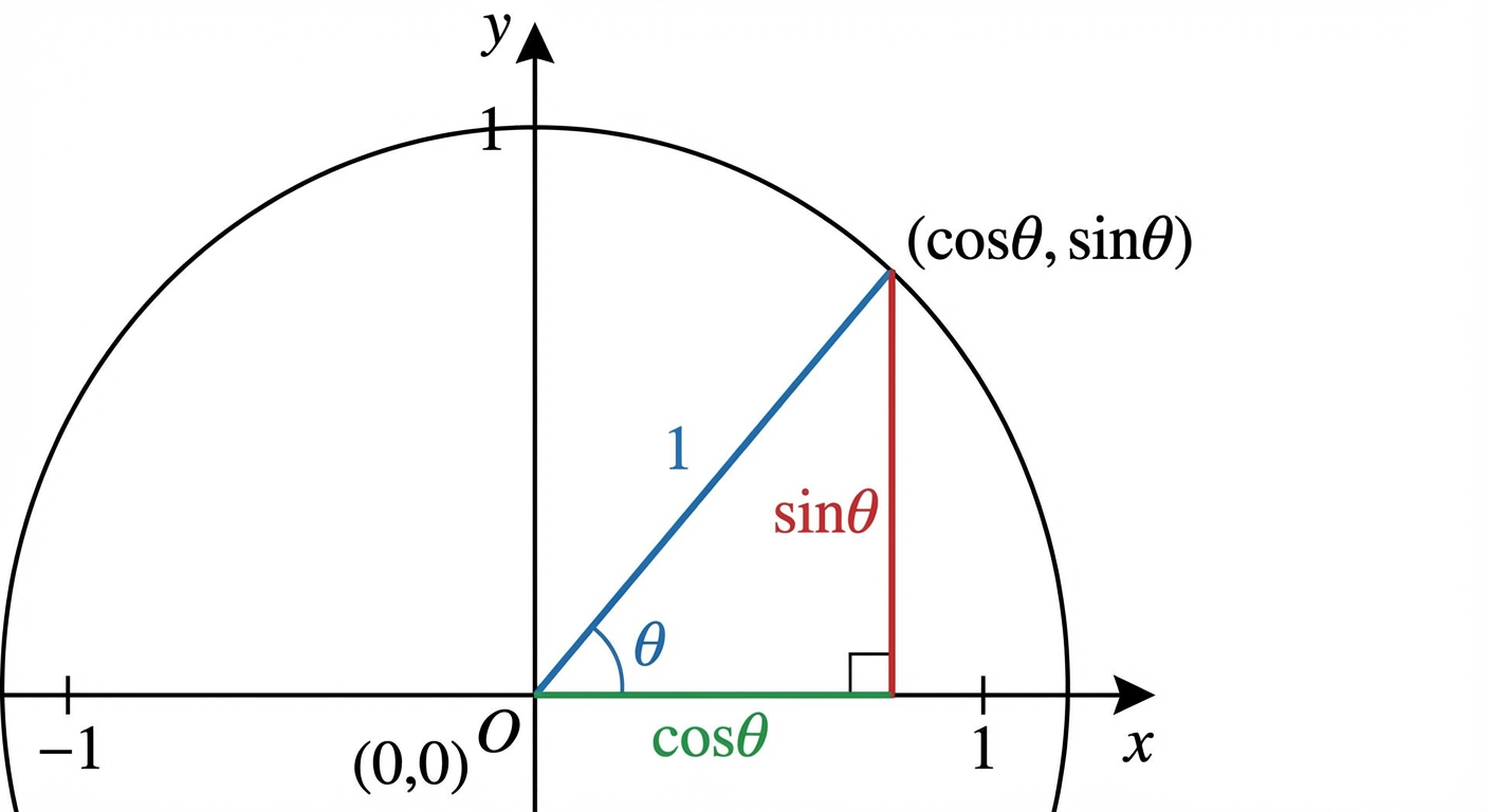
By applying Pythagoras' Theorem () to this triangle, we get , which gives us our identity! This is your go-to move for converting between sine and cosine.
Next, we have the Quotient Identity: . This one is just a clever restatement of SOH CAH TOA. We know and . If you divide them, the 'Hyp' terms cancel out, leaving you with , which is the definition of . Mastering these two identities is non-negotiable. They allow you to take a hideously complicated trig expression and elegantly simplify it, which is exactly what examiners love to test.
Next, we have the Quotient Identity: . This one is just a clever restatement of SOH CAH TOA. We know and . If you divide them, the 'Hyp' terms cancel out, leaving you with , which is the definition of . Mastering these two identities is non-negotiable. They allow you to take a hideously complicated trig expression and elegantly simplify it, which is exactly what examiners love to test.
Worked example
Worked Example: Proving a Trigonometric Identity
Time to Be a Mathematical Detective 🕵️♀️
Prove the identity
- 1Our strategy is to start with the more complex side, the Left-Hand Side (LHS), and manipulate it until it looks like the Right-Hand Side (RHS). The first step here is to combine the two fractions by finding a common denominator, just like you would with numbers.
- 2Now, let's expand the brackets in the numerator. Be careful with the term. The denominator is best left factorised for now, as things might cancel out later.
- 3Look closely at the numerator. Do you see our power couple? We have a term. We can immediately substitute this with 1 using the Pythagorean Identity. This is the key simplification step.
- 4The numerator can now be factorised by taking out a common factor of 2. This is looking promising!
- 5And for the grand finale! The term appears in both the numerator and the denominator, so we can cancel them out. This leaves us with exactly the RHS. We've successfully proven the identity. Mic drop.
Answer
4. Solving Trigonometric Equations in a Given Interval
Alright, let's get into solving trigonometric equations. This is a core skill that's less about memorising formulas and more about solid detective work. Think of it like this: you're given a clue, like , and you need to find all the angles in a specific range (your 'search area', e.g., ) that make this true.
Your first step is always to find the principal value or reference angle. This is the first solution your calculator gives you when you use an inverse function, like . But hold on, that's just one piece of the puzzle! The periodic nature of trig graphs means there are usually multiple solutions. This is where the CAST diagram becomes your best friend.
Your first step is always to find the principal value or reference angle. This is the first solution your calculator gives you when you use an inverse function, like . But hold on, that's just one piece of the puzzle! The periodic nature of trig graphs means there are usually multiple solutions. This is where the CAST diagram becomes your best friend.
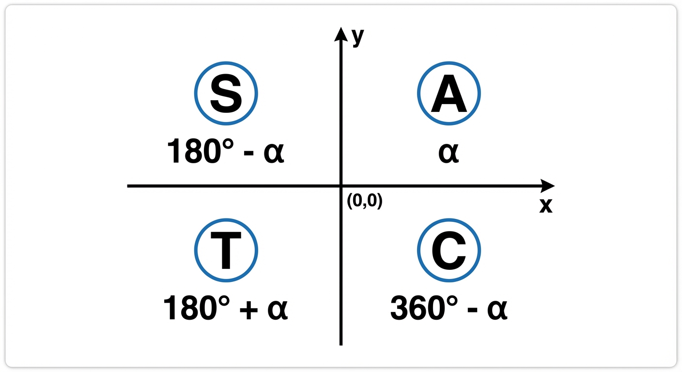
The CAST diagram tells you where the trig functions are positive. For our example, sine is positive, so we look in the 'A' (All) and 'S' (Sin) quadrants. Our principal value, , is the Q1 solution. The Q2 solution is found using the rule , giving us . So, for the interval , our solutions are and . If the value were negative, say , we'd find the principal value for (which is ) and then use the CAST diagram to find solutions in the quadrants where cosine is negative (Q2 and Q3). This skill is fundamental for university-level physics (analysing waves and oscillations) and engineering (signal processing), so mastering this logical process now will pay off massively.
Worked example
Worked Example: Solving a Cosine Equation with a Transformed Angle
Let's Solve This Thing! 💪
Find all solutions for the equation in the interval .
- 1First, let's isolate the cosine term and then adjust our interval to match the angle inside the function, which is . This is a crucial first step to ensure we don't miss any solutions.
- 2Now, let's find the principal value for our new 'angle', which we'll call . We are solving .
- 3Using the CAST diagram, we know that cosine is positive in Quadrant 1 and Quadrant 4. So, we find the second base solution.
- 4We need to find all possible values for within our adjusted interval of . We do this by adding multiples of to our base solutions.
- 5Finally, we substitute back and solve for each value of . Remember to check that your final answers for are within the original interval .
- 6State the final solutions clearly. All four values are valid.
Answer
5. Graphs of Trigonometric Functions
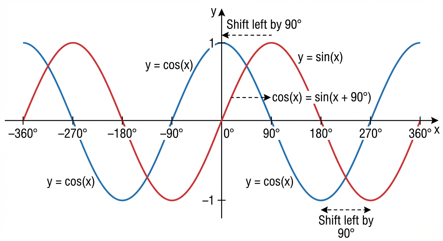
Alright, let's talk about trig graphs. Think of them like the visualisers on a music streaming app – they show the rhythm and flow of a function. The three main artists on our playlist are sine, cosine, and tangent. The sine graph, , is the classic wave. It starts at the origin , vibes up to a maximum height of 1, drops back down, hits a minimum of -1, and then comes back to the start, ready to repeat. This whole cycle is its period, which for sine is (or radians). The 'height' of this wave from its center line is called the amplitude, which is 1 for the basic sine graph.
The cosine graph, , is basically the sine graph's twin, but it started the party a bit earlier. It's what we call phase-shifted. Instead of starting at 0, it starts at its maximum value of 1. It has the same period () and amplitude (1) as sine. It's like they're singing the same song, but one starts on the beat and the other starts a quarter of the way in.
The cosine graph, , is basically the sine graph's twin, but it started the party a bit earlier. It's what we call phase-shifted. Instead of starting at 0, it starts at its maximum value of 1. It has the same period () and amplitude (1) as sine. It's like they're singing the same song, but one starts on the beat and the other starts a quarter of the way in.
Then there's the tangent graph, . This one is the wild card of the group. It shoots up to infinity and reappears from negative infinity, with breaks in between called asymptotes. These are vertical lines the graph gets super close to but never actually touches – like an invisible wall in a video game. These asymptotes happen where the cosine graph would be zero (at , , etc.). The tangent graph repeats its pattern much faster, with a period of only (or radians), and because it goes to infinity, we say it has no amplitude. Understanding these base graphs is key, because soon we'll be giving them a 'glow-up' by stretching, squashing, and shifting them all over the place!
Worked example
Worked Example: Sketching a Transformed Sine Function
Let's Give This Graph a Glow-Up ✨
Sketch the graph of the function for the interval . State the amplitude and the coordinates of any maximum and minimum points in this range.
- 1First, let's identify the transformations from the basic graph. We're looking at the general form . Here, and . This tells us we have a vertical stretch and a vertical shift.
- 2The value of 'a' is 2, which affects the amplitude. The amplitude is . This means our standard cosine wave, which goes between -1 and 1, is now stretched to go between -2 and 2. So, the amplitude is 2.
- 3The value of 'd' is -1. This shifts the entire graph down by 1 unit. The central line moves from the x-axis () down to . This also changes our maximum and minimum values.
- 4Now we can find the coordinates of the max/min points. The basic has maximums at and , and a minimum at . Our transformations don't shift the graph horizontally, so these x-values stay the same.
- 5Finally, let's sketch it! Draw your axes, mark the new central line at , and plot your max and min points. Then, draw the familiar cosine curve shape passing through these points and crossing the central line at and . Done! [IMAGE_PLACEHOLDER_2: A sketch of the graph y = 2cos(x) - 1 from 0 to 360 degrees. The axes should be labelled, with the maximum point (0, 1), minimum point (180, -3), and the central line y=-1 clearly shown.]
Answer
Practice this in the app
Unlock the full chapter: practice questions, flashcards, mock papers and notes, free.
Continue revising