P1: An Introduction to Differentiation
The Magic of Slopes & Turning Points ✨
Introduction
1. Introduction
Welcome to Differentiation! Ever wondered how to find the exact gradient of a curvy line at a single point? That's the core idea we're about to master. We'll kick things off by learning the fundamental power rule, your new best friend for differentiating any polynomial. Then, we'll use that skill to find the equations of tangents and normals to curves – basically, lines that just touch or are perpendicular to a graph at a specific point. The real power move comes next: locating and classifying stationary points. This is how you'll find the exact coordinates of maximums, minimums, and other key features of a function. Finally, we'll dive into connected rates of change, which sounds intense but is just a cool way to see how the rate of change of one variable affects another, like how fast a balloon's radius grows as it's inflated. Let's get started!
2. Differentiation of Powers and the Chain Rule
Alright, let's level up your differentiation game. You're already familiar with the basic power rule for . The brilliant part for A-Levels is that this rule works for any rational number . That means negative powers (like ) and fractional powers (like ) are all fair game. The rule remains the same: bring the power down in front and subtract one from the power. So, . This isn't just an abstract rule; it's the master key to finding the gradient of any point on a curve. The derivative, , is the gradient function.
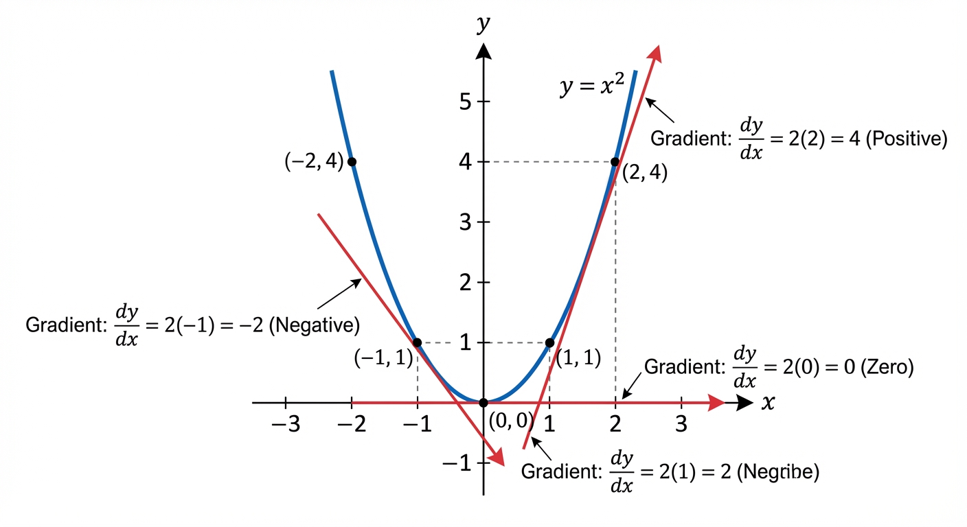
But what happens when you have a function inside another function, like ? This is a composite function, and trying to expand it would be a nightmare. Enter the Chain Rule, your new best friend. Think of it like a Russian doll; you differentiate the outer layer, then multiply by the derivative of the inner layer. For the common case , the shortcut is a lifesaver: you differentiate the 'outside' bracket as normal, and then multiply by the derivative of the 'inside' , which is just . So, . Mastering this is non-negotiable for your exams and is fundamental in university-level physics (for rates of change) and engineering (for optimization problems).
Worked example
Worked Example: Applying the Chain Rule with a Fractional Power
Let's Crack This Problem 🤓
Find the gradient of the curve with equation at the point where .
- 1First things first, we can't differentiate a square root directly. We need to rewrite the equation using index notation. Remember that .
- 2Now we apply the Chain Rule. We'll differentiate the 'outside' function (the power of 1/2) and multiply by the derivative of the 'inside' function . The derivative of is just 6.
- 3Let's simplify that expression. We can multiply the by the 6, and simplify the power.
- 4It's good practice to rewrite the negative fractional power back into a more readable form, using a square root in the denominator. This makes substitution easier.
- 5The question asks for the gradient at the point where x=3. So, we substitute into our derivative function to find the numerical value of the gradient.
Answer
3. Equations of Tangents and Normals to a Curve
Alright, let's get into one of the most classic applications of differentiation: finding tangents and normals. Think of a tangent as a straight line that just kisses a curve at a single point, sharing the exact same gradient at that specific instant. It's like the curve's momentary twin. To find its equation, we need two things: a point and a gradient, . The genius part is that differentiation gives us the gradient! The derivative, , is literally a formula for the gradient of the curve at any point . So, to find the gradient of the tangent () at our point, we just substitute the -coordinate, , into our expression. Once you have the gradient and the point , you just plug them into the good old straight-line equation: .
Now, meet the normal. The normal is the line that is perpendicular to the tangent at that very same point. If the tangent is the high-five, the normal is the line standing at a perfect 90-degree angle to it.
Now, meet the normal. The normal is the line that is perpendicular to the tangent at that very same point. If the tangent is the high-five, the normal is the line standing at a perfect 90-degree angle to it.
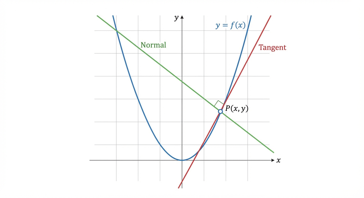
This perpendicular relationship is your key clue. Remember the rule for perpendicular gradients? If the tangent's gradient is , the normal's gradient, , is its negative reciprocal: . The process is almost identical: find the tangent's gradient first, flip it, negate it to get the normal's gradient, and then use the same point to build the equation . Mastering this is not just about acing exams; it's fundamental for physics (think velocity vectors and normal forces) and engineering, setting you up for success at university.
Worked example
Worked Example: Finding the Equation of a Normal
Let's put this theory into practice! 🚀
Find the equation of the normal to the curve at the point where . Give your answer in the form .
- 1First, we need the full coordinates of the point. We're given , so we substitute this into the original equation for the curve to find the corresponding -value.So, our point is .
- 2Next, we need the gradient function. We find this by differentiating the curve's equation with respect to .
- 3Now, we find the gradient of the tangent at our specific point by substituting into our derivative.The gradient of the tangent at is 4.
- 4The normal is perpendicular to the tangent. So, we find the negative reciprocal of the tangent's gradient to get the gradient of the normal, .
- 5Finally, we use the point and the normal's gradient in the straight-line equation formula, , and rearrange it into the required form.
Answer
4. Locating and Classifying Stationary Points
Alright, let's talk stationary points. Think of them as the peaks and valleys on a graph – the moments where the curve is momentarily flat. At these points, the gradient is zero. So, your first step is always to find the first derivative, , and solve the equation . This will give you the x-coordinates of all the 'flat spots'.
But finding them is only half the battle. For your exam, you need to classify their nature: is it a peak (local maximum), a valley (local minimum), or a stationary point of inflection?
But finding them is only half the battle. For your exam, you need to classify their nature: is it a peak (local maximum), a valley (local minimum), or a stationary point of inflection?
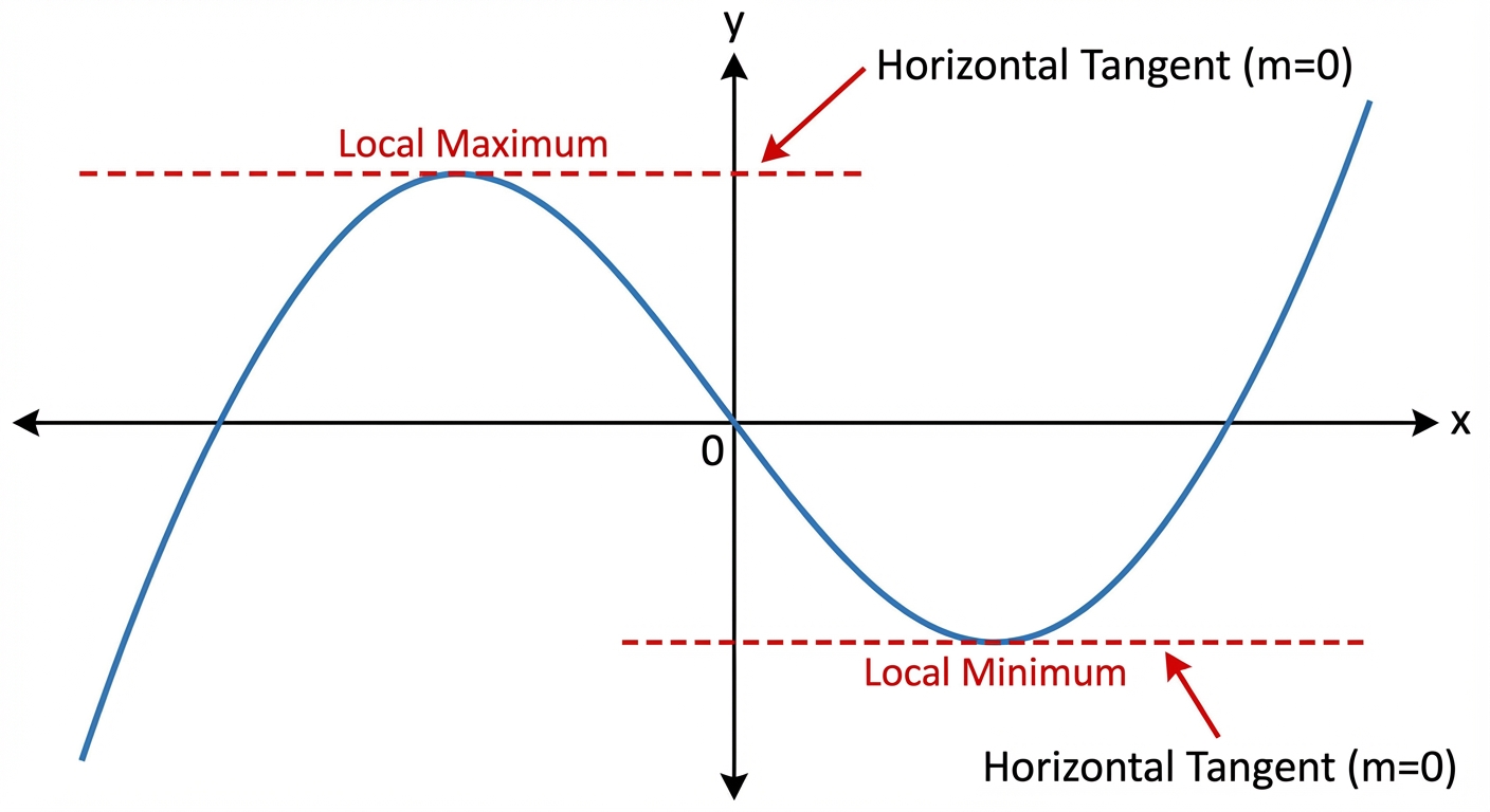
Your go-to tool for this is the second derivative test. The second derivative, , tells us about the curve's curvature. Once you have the x-coordinate of a stationary point, plug it into the second derivative:
- If , the curve is concave up (like a smiley face 😊), so you've found a local minimum.
- If , the curve is concave down (like a frowny face ☹️), indicating a local maximum.
- If , the test is inconclusive. You must then check the sign of the gradient () just before and after the point to classify it. This isn't just abstract maths; it's the core of optimisation used in economics to maximise profit or in engineering to minimise material waste. Getting this down is a massive step up in your mathematical maturity.
- If , the curve is concave up (like a smiley face 😊), so you've found a local minimum.
- If , the curve is concave down (like a frowny face ☹️), indicating a local maximum.
- If , the test is inconclusive. You must then check the sign of the gradient () just before and after the point to classify it. This isn't just abstract maths; it's the core of optimisation used in economics to maximise profit or in engineering to minimise material waste. Getting this down is a massive step up in your mathematical maturity.
Worked example
Worked Example: Analysis of a Cubic Function
Let's put this theory into practice! 🚀
Find the coordinates of the stationary points on the curve and determine their nature.
- 1First, we need the gradient function, . Differentiating the original function gives us the formula for the gradient at any point .
- 2Stationary points occur where the gradient is zero. So, we set our derivative equal to zero and solve for . This is a standard quadratic equation.
- 3We need the full coordinates, so we substitute these x-values back into the original equation for . Don't accidentally use the derivative!
- 4To classify the points using the second derivative test, we first need to find the second derivative, . We just differentiate our first derivative.
- 5Now for the final verdict. We substitute each x-coordinate into the second derivative. A positive result means it's a minimum; a negative result means it's a maximum.
Answer
5. Application of the Chain Rule to Connected Rates of Change
Alright, let's get into one of the coolest applications of differentiation: Connected Rates of Change. Think of it like this: you're scrolling through social media, and you know the rate your battery is draining per minute. But what you really want to know is how fast your screen time is increasing. These two things—battery drain and screen time—are connected, right? That's the core idea here. In maths, when we have two variables, say and , that are linked by an equation (like the volume and radius of a sphere), their rates of change with respect to a third variable (almost always time, ) are also linked.
The magic formula that connects everything is a slick application of the chain rule: This equation is your absolute best friend for these problems. Let's break it down:
• is the rate of change of with respect to time (this is usually what you're asked to find).
• is the rate of change of with respect to time (this is usually given to you in the problem).
• is the 'connector'. It's the derivative of your original equation that links and . You'll calculate this yourself.
The magic formula that connects everything is a slick application of the chain rule: This equation is your absolute best friend for these problems. Let's break it down:
• is the rate of change of with respect to time (this is usually what you're asked to find).
• is the rate of change of with respect to time (this is usually given to you in the problem).
• is the 'connector'. It's the derivative of your original equation that links and . You'll calculate this yourself.
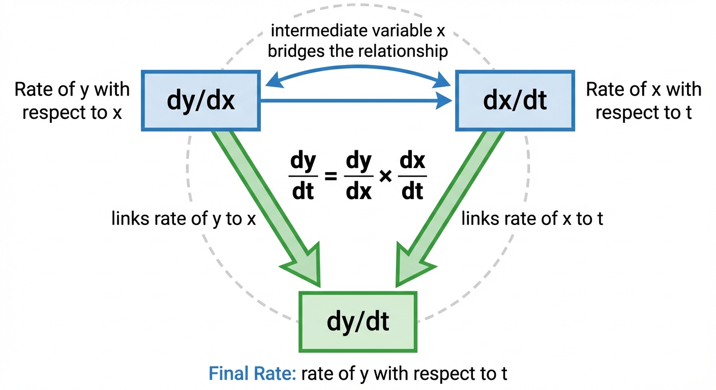
It's super useful to think of the terms 'cancelling out' to help you remember the formula. Technically they aren't fractions, but it's a brilliant mental shortcut that the examiners are totally cool with. Mastering this isn't just about acing P1; this concept pops up everywhere in physics, engineering, and economics at university. It’s how you model real-world dynamic systems. So, let's nail it down!
Worked example
Worked Example: Rate of Change of a Spherical Balloon's Volume
Let's blow this problem up! 🎈
Air is being pumped into a spherical balloon at a constant rate of . Find the rate at which the radius of the balloon is increasing when its radius is . The volume of a sphere with radius is given by .
- 1First, let's identify what we know and what we need to find. We're given the rate of change of volume with respect to time, and we need to find the rate of change of the radius with respect to time.
- 2We need the 'connector' derivative that links and . We're given the formula for the volume of a sphere, so let's differentiate with respect to .
- 3Now we can set up our connected rates of change formula using the variables , , and . We'll use the chain rule to link the rates.
- 4We want to find , so let's rearrange the formula to make it the subject. Then, we can substitute in the values we know. We need to calculate at the specific instant when .
- 5Finally, substitute the given value for and our calculated value for into the rearranged formula to solve for . Don't forget the units!
Answer
Practice this in the app
Unlock the full chapter: practice questions, flashcards, mock papers and notes, free.
Continue revising