S2 - Hypothesis Tests
The Procedure for Hypothesis Testing
1. The Procedure for Hypothesis Testing
Alright, let's break down hypothesis testing. Think of it as being a detective for data. You have a claim (like a game dev saying a patch doesn't increase lag), and you want to see if there's enough evidence to call them out.
First up, we have our two competing theories, the hypotheses:
1. The Null Hypothesis (): This is the boring, 'status quo' or 'no change' idea. It's the default assumption. For the game patch, would be: The lag has not changed. It's what we assume is true until proven otherwise.
2. The Alternative Hypothesis (): This is the spicy new theory you're investigating. It's what you suspect might be true instead. It could be that the lag has increased (a one-tailed test), or that it has simply changed (increased or decreased, a two-tailed test).
Next, we set the Significance Level (). This is basically your 'doubt threshold'. It's usually small, like 5% (0.05) or 1% (0.01). If you set , you're saying: 'I'm only going to reject the null hypothesis if the result I see is so weird it would only happen by chance less than 5% of the time.' It’s the risk you're willing to take of making the wrong call.
Now, we collect our data (play some games) and calculate the Test Statistic. This is a single number that summarizes our sample evidence. It's the key piece of data we'll use to make our decision.
So, how do we decide? We use the significance level to find the Critical Region (or Rejection Region). This is the 'danger zone' of extreme values. If our test statistic falls into this region, it's considered strong evidence against .
First up, we have our two competing theories, the hypotheses:
1. The Null Hypothesis (): This is the boring, 'status quo' or 'no change' idea. It's the default assumption. For the game patch, would be: The lag has not changed. It's what we assume is true until proven otherwise.
2. The Alternative Hypothesis (): This is the spicy new theory you're investigating. It's what you suspect might be true instead. It could be that the lag has increased (a one-tailed test), or that it has simply changed (increased or decreased, a two-tailed test).
Next, we set the Significance Level (). This is basically your 'doubt threshold'. It's usually small, like 5% (0.05) or 1% (0.01). If you set , you're saying: 'I'm only going to reject the null hypothesis if the result I see is so weird it would only happen by chance less than 5% of the time.' It’s the risk you're willing to take of making the wrong call.
Now, we collect our data (play some games) and calculate the Test Statistic. This is a single number that summarizes our sample evidence. It's the key piece of data we'll use to make our decision.
So, how do we decide? We use the significance level to find the Critical Region (or Rejection Region). This is the 'danger zone' of extreme values. If our test statistic falls into this region, it's considered strong evidence against .
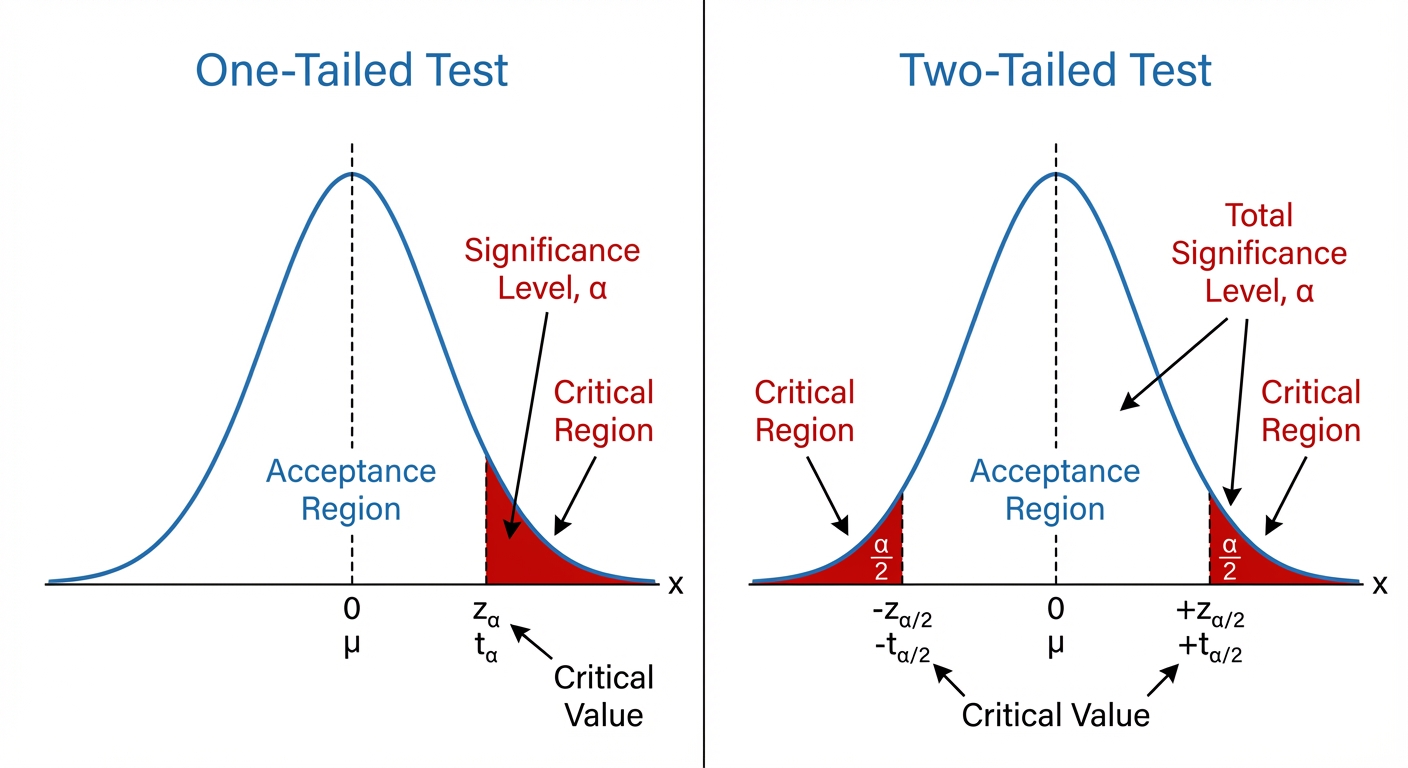
If your test statistic lands in the shaded area, you've got drama! You reject . If it lands in the main, unshaded part, you don't have enough evidence, so you do not reject . Notice we never say 'accept' – we just say we lack the evidence to throw it out. It’s like a jury saying 'not guilty' instead of 'innocent'.
Worked example
Worked Example: Hypothesis Test for a Binomial Proportion
Is This TikTok Ad *Really* Working? 🧐
A marketing agency claims that a new TikTok ad format will have a click-through rate of 25%. The client thinks this is an overestimate. To test the claim, the ad is shown to 40 randomly selected users, and only 5 of them click on it. Test the agency's claim at the 5% significance level.
- 1First, we define our hypotheses. The null hypothesis () is the agency's claim. The alternative hypothesis () is the client's suspicion that the rate is lower. Let be the true click-through rate.
- 2We are counting the number of 'successes' (clicks) in a fixed number of trials (users), so this fits a binomial distribution. Our test statistic, , is the number of clicks from 40 users.
- 3Now we find the critical region. Since is , this is a one-tailed test. We're looking for an unusually low number of clicks. We need to find the critical value such that the probability of getting or fewer clicks is less than our 5% significance level.
- 4We compare our observed result (the test statistic) from the sample to the critical region we just found.
- 5Our observed value of 5 falls inside the critical region (). This means our result is statistically significant and gives us enough evidence to reject the null hypothesis.
- 6Finally, we state our conclusion in the context of the original problem about the TikTok ad.There is sufficient evidence at the 5% significance level to reject the agency's claim and conclude that the click-through rate is lower than 25%.
Answer
There is sufficient evidence at the 5% significance level to reject the agency's claim and conclude that the click-through rate is lower than 25%.
2. Hypothesis Tests for a Population Mean with Known Variance
Alright, let's get into it. Imagine a company like Spotify claims the average listening time for a premium user is 3 hours a day. You and your friends think it's way higher. How do you test that claim? This is where the Z-test for a population mean comes in, and it's our first major tool for hypothesis testing.
The key condition here is that we know the population variance, (or the standard deviation, ). This is a bit of a perfect-world scenario, like a game dev knowing the exact variance in player reaction times from millions of data points. When we know AND the original population is normally distributed, the sample mean, , will also be perfectly normally distributed. Its distribution is .
But what if the original population isn't normal? Maybe it's skewed. This is where a super-important idea called the Central Limit Theorem (CLT) saves the day. The CLT says that if your sample size () is large enough (a good rule of thumb is ), the distribution of the sample means () will be approximately normal, no matter what the original population looked like! This is clutch because it means we can still use the Normal distribution for our test. It’s like taking a screenshot of a chaotic Snapchat story; if you take enough screenshots over time, the average 'vibe' starts to look pretty predictable.
To actually run the test, we calculate a test statistic. For this scenario, it's the Z-statistic. The formula is your new best friend:
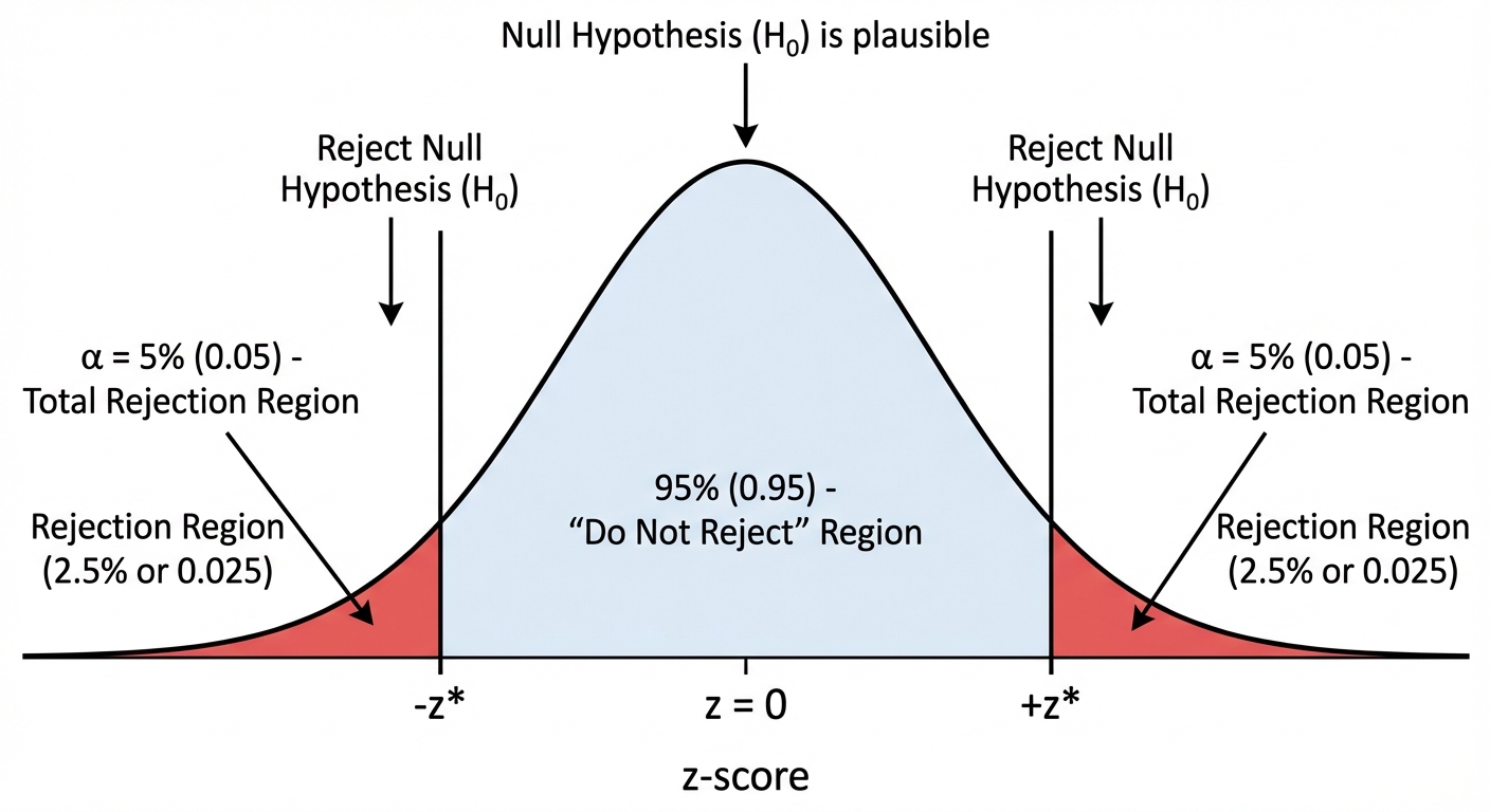
Let's break it down: is the mean from your sample (the evidence you collected). is the mean from the null hypothesis (the original claim you're testing). The denominator, , is the standard error, which measures the typical variation we'd expect between sample means. Essentially, the Z-score tells us how many standard errors our sample mean is away from the claimed population mean. A big Z-score (either positive or negative) suggests our sample result is pretty unusual if the original claim is true, which might lead us to reject it.
The key condition here is that we know the population variance, (or the standard deviation, ). This is a bit of a perfect-world scenario, like a game dev knowing the exact variance in player reaction times from millions of data points. When we know AND the original population is normally distributed, the sample mean, , will also be perfectly normally distributed. Its distribution is .
But what if the original population isn't normal? Maybe it's skewed. This is where a super-important idea called the Central Limit Theorem (CLT) saves the day. The CLT says that if your sample size () is large enough (a good rule of thumb is ), the distribution of the sample means () will be approximately normal, no matter what the original population looked like! This is clutch because it means we can still use the Normal distribution for our test. It’s like taking a screenshot of a chaotic Snapchat story; if you take enough screenshots over time, the average 'vibe' starts to look pretty predictable.
To actually run the test, we calculate a test statistic. For this scenario, it's the Z-statistic. The formula is your new best friend:
Let's break it down: is the mean from your sample (the evidence you collected). is the mean from the null hypothesis (the original claim you're testing). The denominator, , is the standard error, which measures the typical variation we'd expect between sample means. Essentially, the Z-score tells us how many standard errors our sample mean is away from the claimed population mean. A big Z-score (either positive or negative) suggests our sample result is pretty unusual if the original claim is true, which might lead us to reject it.
Worked example
Worked Example: Z-Test for a Population Mean
Is the Battery Life a Lie? 🔋
A phone manufacturer claims their new model has an average battery life of hours for continuous video playback. The battery life is known to be normally distributed with a standard deviation of hours. A tech reviewer tests a random sample of phones and finds their average battery life is hours. Test, at the 5% significance level, whether the average battery life is greater than the manufacturer's claim.
- 1First, we set up our null () and alternative () hypotheses. is the original claim (the 'status quo'). is what the reviewer suspects. Since they're testing if the battery life is greater than the claim, it's a one-tailed test.
- 2Next, we find the critical value for our significance level. We have a 5% significance level () and a one-tailed test. We need to find the Z-score that marks the top 5% of the normal distribution. Using tables or a calculator's inverse normal function (invNorm(0.95)), we find this value.
- 3Now it's time to calculate our test statistic using the Z-formula. We plug in our sample mean (), the claimed population mean (), the population standard deviation (), and the sample size ().
- 4Let's make a decision. We compare our calculated Z-statistic to our critical value. We can see that . This means our result falls into the rejection region.
- 5Finally, we write a conclusion in the context of the problem. Don't just say 'reject H0'. What does it actually mean for the phones? It means we found enough evidence to support the reviewer's suspicion.
Answer
3. Type I and Type II Errors
Okay, so you've run your hypothesis test, you've got your p-value, and you've made a conclusion. But what if... you're wrong? 😱 It happens! Hypothesis testing is all about probability, not certainty. Think of it like a court case. The null hypothesis, , is 'the defendant is innocent'. We only reject this if we have strong evidence they're guilty. A Type I Error is like convicting an innocent person. It's when we reject a null hypothesis that was actually TRUE. We found a statistically significant result, but it was just a fluke, a one-in-a-million chance (or, more likely, a one-in-twenty chance!). The probability of making a Type I error is literally the significance level of the test, which we call . So if you set your significance level to 5% (), you're accepting there's a 5% chance you'll make this kind of mistake. It's the risk you're willing to take.
Then there's the Type II Error. This is the opposite: it's like letting a guilty person walk free. It's when we fail to reject a null hypothesis that is actually FALSE. Our test wasn't sensitive enough to pick up on the change. Maybe your friend did get better at that video game, but their scores in your sample weren't quite good enough to prove it. The probability of this error is called . Calculating is a bit different because you need to know the true value of the parameter to see how often you'd miss it. For example, 'If the true mean is actually 105, what's the probability our test fails to notice it's not 100?'.
Then there's the Type II Error. This is the opposite: it's like letting a guilty person walk free. It's when we fail to reject a null hypothesis that is actually FALSE. Our test wasn't sensitive enough to pick up on the change. Maybe your friend did get better at that video game, but their scores in your sample weren't quite good enough to prove it. The probability of this error is called . Calculating is a bit different because you need to know the true value of the parameter to see how often you'd miss it. For example, 'If the true mean is actually 105, what's the probability our test fails to notice it's not 100?'.
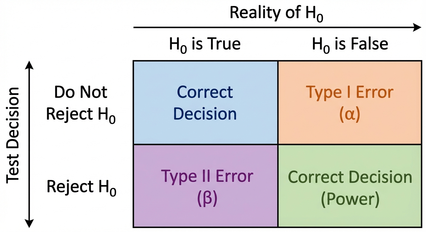
Finally, let's talk about the Power of a test. This is the cool one. Power is the probability that you correctly reject a false null hypothesis. It's the test's ability to detect an effect when there really is one. Think of it as your test's 'rizz' – its ability to successfully spot the truth. The Power is calculated as . A powerful test has a low chance of making a Type II error. You want a test with high power, just like you want a phone with a good signal!
Worked example
Worked Example: Calculating Error Probabilities in a Binomial Test
Let's Check This Gamer's Claim 🎮
A gamer claims her success rate in a specific level is 20%. Her friend suspects the rate is actually higher. To test this, the friend observes 20 games. The test is conducted at the 5% significance level. The critical region is found to be , where is the number of successes.
a) Calculate the actual significance level (the probability of a Type I error).
b) Find the probability of a Type II error if the gamer's true success rate is actually 40%.
a) Calculate the actual significance level (the probability of a Type I error).
b) Find the probability of a Type II error if the gamer's true success rate is actually 40%.
- 1First, let's define our hypotheses and the distribution. The null hypothesis () is the gamer's claim, and the alternative () is the friend's suspicion. Under , the number of successes follows a Binomial distribution with and .
- 2For part (a), we need to find the probability of a Type I error. This is the probability of rejecting when it's true. We reject if our result falls in the critical region (). So, we calculate this probability using the distribution from (where ). This is also called the actual significance level.
- 3For part (b), we calculate the probability of a Type II error. This is when we fail to reject when it's actually false. We fail to reject if we are in the 'acceptance region', which is the opposite of the critical region (). The question tells us to assume the true probability of success is now . So, we must recalculate our probability using this new value for .
- 4Now we find the probability of landing in the acceptance region () using the new, true distribution where . This probability is .
- 5Bonus round! Let's find the power of this test (for the alternative ). The power is the probability of correctly rejecting the false . It's simply .
Answer
4. Hypothesis Tests for Binomial and Poisson Distributions
Alright, let's dive into hypothesis tests for Binomial and Poisson distributions. Think of it like this: a game developer claims a rare item has a 10% drop rate (). You grind for hours, defeat 50 enemies (), and get the item only twice. Is the drop rate claim legit, or did they nerf it? That's what we're testing!
We have two main ways to tackle these problems: direct evaluation or using a Normal approximation.
Direct Evaluation: This is our go-to when the numbers are pretty small (for Binomial, if or is less than 5; for Poisson, if is less than 15). We calculate the probability of getting our observed result, or something even more extreme. This is the p-value. If this probability is super tiny (smaller than our significance level, , usually 5%), it's like getting a mythic weapon on your first try – so unlikely that we suspect the original claim () is wrong.
We can also think in terms of a Critical Region. This is the 'rejection zone' of outcomes. For discrete data, it’s a bit quirky. We can't land exactly on a 5% probability. We find the first value where the cumulative probability dips below our significance level.
We have two main ways to tackle these problems: direct evaluation or using a Normal approximation.
Direct Evaluation: This is our go-to when the numbers are pretty small (for Binomial, if or is less than 5; for Poisson, if is less than 15). We calculate the probability of getting our observed result, or something even more extreme. This is the p-value. If this probability is super tiny (smaller than our significance level, , usually 5%), it's like getting a mythic weapon on your first try – so unlikely that we suspect the original claim () is wrong.
We can also think in terms of a Critical Region. This is the 'rejection zone' of outcomes. For discrete data, it’s a bit quirky. We can't land exactly on a 5% probability. We find the first value where the cumulative probability dips below our significance level.
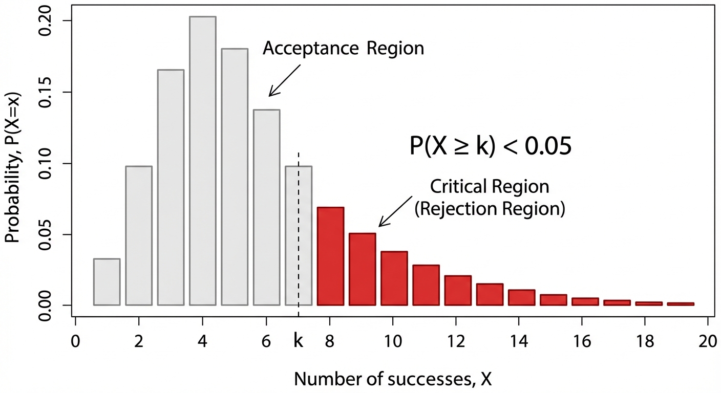
. Any result in this zone means we reject .
Normal Approximation: When the numbers get big, calculating exact probabilities is a nightmare. So, we 'cheat' and use the Normal distribution. It's like using a high-res texture pack to smooth out a blocky game world. The one HUGE thing to remember is the continuity correction. Since we're using a continuous model for discrete data, we have to adjust by 0.5. So becomes in our Normal model. Forgetting this is the number one way to lose marks! 😬
Normal Approximation: When the numbers get big, calculating exact probabilities is a nightmare. So, we 'cheat' and use the Normal distribution. It's like using a high-res texture pack to smooth out a blocky game world. The one HUGE thing to remember is the continuity correction. Since we're using a continuous model for discrete data, we have to adjust by 0.5. So becomes in our Normal model. Forgetting this is the number one way to lose marks! 😬
Worked example
Worked Example: Hypothesis Test for a Binomial Proportion
Did the Training Actually Work? 🤔
A student working at a café is told that the probability of a customer ordering the new 'Cosmic Frappé' is 0.1. After promoting it heavily for a week, they believe the probability has increased. In the next 40 customers, 7 order the drink. Test, at the 5% significance level, whether there is evidence that the promotion was effective.
- 1First, we set up our null hypothesis (), which is the 'no change' scenario, and our alternative hypothesis (), which is what we're trying to prove. We'll define our random variable and its distribution assuming is true. Since we have a fixed number of trials (40 customers) and a constant probability of success, this is a Binomial distribution.
- 2Before we dive in, we should check if we can use a Normal approximation. We calculate . If it's less than 5, we must use the exact Binomial distribution.
- 3We observed 7 successes. Since our alternative hypothesis is , this is an upper one-tailed test. We need to find the probability of getting our result (7) or something even more extreme (more than 7). So, we calculate . It's easier to calculate this using the complement: .
- 4Now we compare our calculated p-value with the significance level, , which was given as 5% or 0.05. If the p-value is less than , we reject . If it's greater, we don't.
- 5Our p-value is greater than the significance level. This means our result is not 'surprising' enough to reject the null hypothesis. We conclude by stating what this means in the context of the café problem.
Answer
Practice this in the app
Unlock the full chapter: practice questions, flashcards, mock papers and notes, free.
Continue revising