Chapter P1: Integration
Integration: The Ultimate Undo Button! ⏪
Introduction
1. Introduction
Alright, let's tackle Integration! If you thought differentiation was cool for finding gradients, get ready for its awesome sibling. Integration is essentially the reverse process, and it's a powerhouse tool in your A-Level toolkit. We'll start by learning how to 'undo' differentiation with Indefinite Integration. Then, we'll give it boundaries with Definite Integration to find specific numerical values. Why? Because that unlocks the magic of finding the exact Area Under a Curve, a trick that seems impossible until you see how it's done. Finally, we'll take that 2D area, spin it around an axis, and calculate the Volume of Revolution to create 3D shapes. It might sound like a lot, but we'll break it down step-by-step. You've got this! 💪
2. Indefinite Integration and the Constant of Integration
Alright, let's get into it. Think of differentiation as finding the gradient function of a curve. Indefinite integration is the exact opposite – it's the process of finding the original function when you've been given the gradient. It’s like having the answer to a puzzle and needing to figure out the original question. The fundamental rule for integrating a term like is to add one to the power, then divide by the new power. So, . But wait, what's that mysterious '' crashing the party? This is the constant of integration, and it's absolutely crucial for your exams. Remember how differentiating a constant term (like +5 or -20) makes it vanish? Well, when we integrate, we have no idea if there was a constant there to begin with. The '' is our placeholder for that unknown value. Integrating a gradient function like gives us a whole family of possible curves, like , , etc., all with the same gradient.
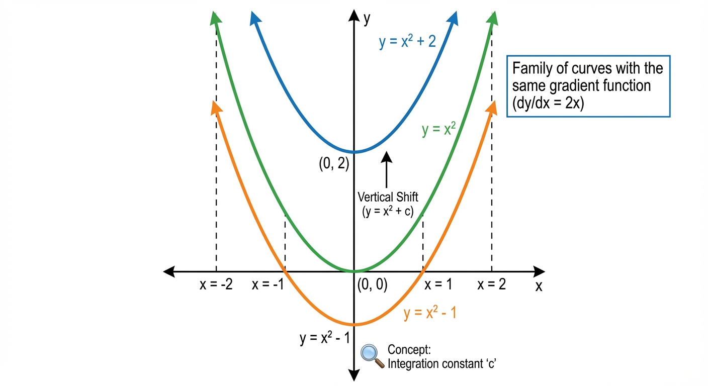
For your A-Level syllabus, you need to master integrating expressions in the form . The rule is a slight extension of the basic one: . Notice we still add one to the power and divide by the new power, but we also divide by 'a', which is the derivative of the inner function . This is essentially the reverse of the chain rule. To nail down the specific value of C and find the unique equation of a curve, you'll be given a coordinate that the curve passes through. You substitute this pair into your integrated equation and solve for C. This skill isn't just for exams; it's fundamental in physics for finding displacement from velocity, in economics for calculating total cost from marginal cost, and in engineering for various modelling scenarios. Mastering this sets a strong foundation for more advanced calculus you'll encounter at university.
Worked example
Worked Example: Finding the Equation of a Curve
Solving the Mystery of the Missing Constant! 🕵️♂️
The gradient of a curve is given by the expression . Given that the curve passes through the point P(3, 10), find the equation of the curve.
- 1First things first, to find the equation of the curve, , we need to integrate the gradient function, . Let's set up the integral.
- 2Now we apply the integration rule for , which is . Here, our constant multiple is 6, , , and . Don't forget the constant of integration, !
- 3Let's simplify that expression. The denominator becomes . This will cancel out nicely with the 6 at the front.
- 4We have the general solution. To find the specific solution for our curve, we use the given point P(3, 10). Substitute and into the equation to find the value of C.
- 5Finally, solve for C and write down the complete, unique equation for the curve. This is your final answer, so present it clearly.
Answer
3. Evaluating Definite Integrals
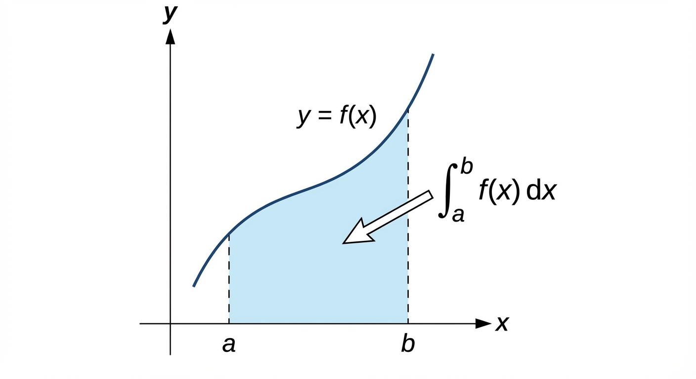
Alright, let's level up from indefinite integration. Think of indefinite integration as getting the general formula for a journey, but definite integration is like finding the exact distance you travelled between two specific mile markers. That's the core idea here. A definite integral, written as , calculates a specific numerical value. The numbers and are called the limits of integration, with being the lower limit and the upper limit. They define the exact interval on the x-axis we care about.
The magic behind evaluating this is the Fundamental Theorem of Calculus. It's a game-changer and a cornerstone of university-level maths. It states that if you integrate to get , then the value of the definite integral is simply . We write this as . Notice something missing? The '+ C'! When you calculate , the constants cancel out, which is super convenient. You're finding the net change in the antiderivative across the interval.
The magic behind evaluating this is the Fundamental Theorem of Calculus. It's a game-changer and a cornerstone of university-level maths. It states that if you integrate to get , then the value of the definite integral is simply . We write this as . Notice something missing? The '+ C'! When you calculate , the constants cancel out, which is super convenient. You're finding the net change in the antiderivative across the interval.
We also need to touch on improper integrals, which will give you a taste of first-year university calculus. This is where one of the limits is infinity, like . You can't just 'plug in' infinity, so we use a clever trick with limits. We evaluate the integral from to some variable, let's say , and then find the limit as . This helps us determine if an infinitely long area actually converges to a finite number, which is a mind-bending but powerful concept used in fields like quantum mechanics and probability theory.
Worked example
Worked Example: Evaluating a Definite Integral with Fractional Powers
Let's Get This Bread (and this answer) 🍞
Calculate the exact value of the definite integral .
- 1First things first, we need to rewrite the integrand into a form we can easily integrate using the power rule. Remember that is , so is . This prep work is crucial for avoiding mistakes.
- 2Now, let's integrate each term with respect to . For , the power increases from 1 to 2. For , the power increases from -1/2 to 1/2. We'll put the result in square brackets with the limits, ready for evaluation.
- 3Before substituting the limits, let's simplify the expression inside the brackets. Dividing by is the same as multiplying by 2. It's also helpful to convert back to to make the arithmetic clearer.
- 4Time to apply the Fundamental Theorem of Calculus: . We substitute the upper limit () into our simplified expression, and then subtract the result of substituting the lower limit ().
- 5Finally, we just need to do the arithmetic. Be careful with your brackets and signs here! This gives us the final numerical value of the definite integral.
Answer
4. Calculating Areas Bounded by Curves and Axes
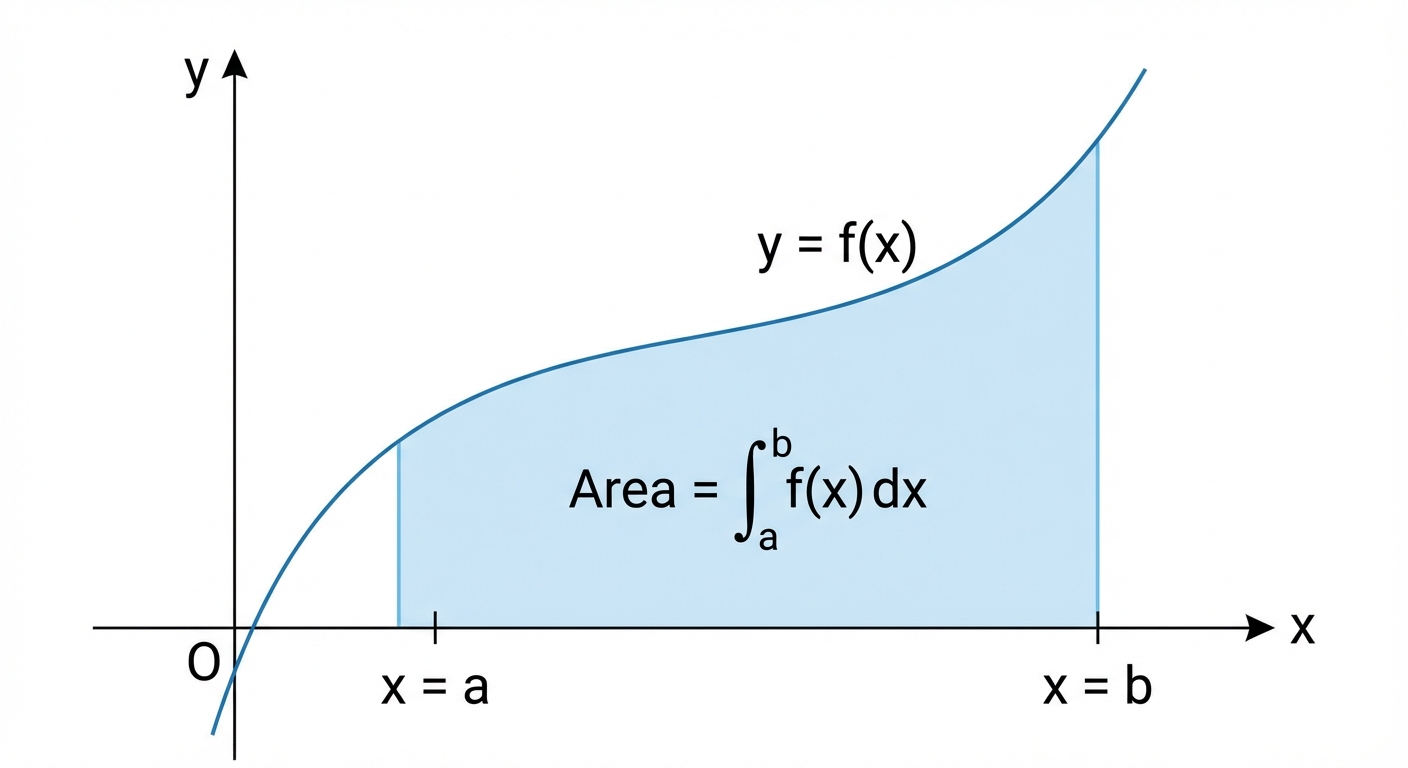
Alright, let's get into one of the coolest applications of integration: finding the area under a curve. Seriously, this isn't just abstract math; it's the foundation for calculating everything from the trajectory of a rocket to the total revenue a company makes over time. The core idea is that a definite integral, , represents the exact area trapped between the curve , the x-axis, and the vertical lines and . Think of it as summing up an infinite number of super-skinny rectangular strips under the curve to get a perfect measurement.
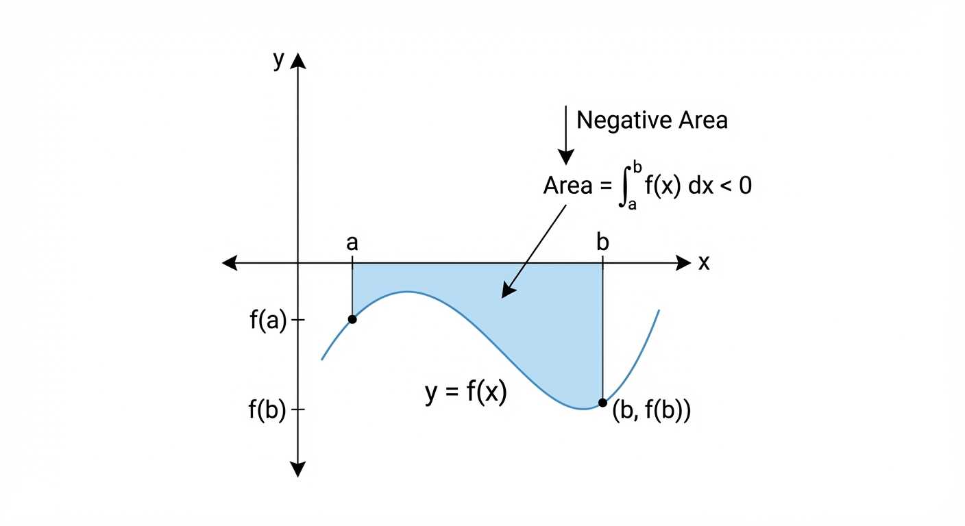
Now, here's the first exam-level trap you need to watch out for: negative areas. If your curve dips below the x-axis, the integral for that section will give you a negative value. But can you have negative physical space? Nope. So, if you're asked for the area, you must treat that value as positive. You can either take the absolute value of the negative result, or calculate for that part.
The real A-Level challenge comes when finding the area between two curves, say and . The strategy is simple but powerful: find the area under the top curve and subtract the area under the bottom curve. This simplifies to a single integral: . The trickiest part is often finding the limits of integration, and . You'll usually need to find the points where the curves intersect by setting their equations equal to each other and solving for . This skill is crucial for university-level calculus in engineering, physics, and economics. Mastering this is a direct investment in your future studies! 🚀
Worked example
Worked Example: Area Bounded by a Curve and a Line
Let's Solve This Thing! 🚀
Find the exact area of the finite region bounded by the curve and the line .
- 1First things first, we need to find where the curve and the line meet. These intersection points will be our limits of integration, and . We do this by setting the two equations equal to each other and solving the resulting quadratic.
- 2Now we know our limits are and . We need to set up the integral for the area between the curves. The formula is . In this region, the quadratic curve is above the line (check by testing a point like ).
- 3Let's simplify the expression inside the integral before we start integrating. This makes life way easier and reduces the chance of errors.
- 4Time to integrate! We apply the power rule for integration, , to each term in our simplified polynomial.
- 5This is the final step – the evaluation. We substitute the upper limit () into our integrated expression, then subtract the result of substituting the lower limit (). Be super careful with your signs here!
Answer
5. Volumes of Revolution
Alright, let's level up our integration game. You know how we can find the area under a curve, right? That's like finding the space a 2D shape takes up. A Volume of Revolution is what happens when you take that 2D area and spin it around an axis, like a potter's wheel or a record player. Think of it like this: you sketch a cool profile for a custom vase on paper. If you could rotate that 2D sketch around the y-axis, you'd get the actual 3D vase! That's what we're calculating here.
The core idea is to slice the 3D shape into an infinite number of super-thin discs, like a stack of coins. The volume of one disc is . In our case, the radius is just the function's value ( if we rotate around the x-axis, or if we rotate around the y-axis), and the height is an infinitesimally small change, or . To get the total volume, we just add up all these tiny discs using integration!
The core idea is to slice the 3D shape into an infinite number of super-thin discs, like a stack of coins. The volume of one disc is . In our case, the radius is just the function's value ( if we rotate around the x-axis, or if we rotate around the y-axis), and the height is an infinitesimally small change, or . To get the total volume, we just add up all these tiny discs using integration!
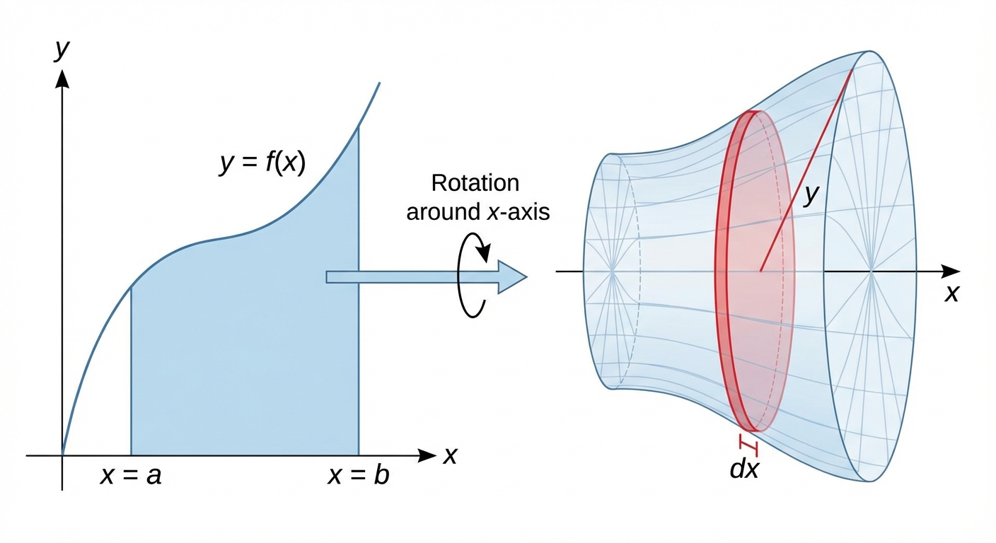
So, to find the volume when a curve is rotated about the x-axis between and , the formula is: What if the shape is hollow, like a donut or a lampshade? This happens when the region we're rotating is bounded by two curves, say an 'outer' curve and an 'inner' curve . It's like making the big solid shape and then drilling out the middle. You just calculate the volume of the outer shape and subtract the volume of the inner one. The formula becomes: This is super powerful – you can find the volume of almost any symmetrical 3D object you can think of, from a rocket nose cone to a custom wheel rim. It's basically 3D printing with math. 😉
Worked example
Worked Example: Volume of a Solid with a Hollow Core
Let's Make a 3D Donut with Math 🍩
The region is bounded by the curve and the line . Find the volume of the solid formed when region is rotated through about the y-axis.
- 1First up, we need to rearrange our equations to make the subject, since we're rotating around the y-axis. This means we'll be integrating with respect to . The line is our outer boundary, and the curve is our inner boundary. We also need our limits of integration for . The region starts where the curve begins on the y-axis (when , ) and ends at the line . So our limits are from 2 to 6.Rearrange the curve: .
Limits of integration: from (vertex of the curve) to (the horizontal line). - 2Okay, let's set up the integral. Since we're rotating around the y-axis, our formula is . We already have in terms of from our curve, and our limits are and .
- 3Now for the fun part: integration! We apply the power rule to integrate with respect to . Remember, integrating gives and integrating a constant gives the constant times .
- 4Finally, we substitute our limits into the integrated expression. We plug in the upper limit (6), then subtract the result of plugging in the lower limit (2). Be careful with your brackets and signs here!
- 5And we're done! The volume of the solid is cubic units. Don't forget the units if the question asks for them. Nailed it! 🎉Final Answer: The volume is cubic units.
Answer
Final Answer: The volume is cubic units.
Practice this in the app
Unlock the full chapter: practice questions, flashcards, mock papers and notes, free.
Continue revising