Chapter P1: Coordinate Geometry
Lines, Circles, and Where They Meet! 📐✨
Introduction
1. Introduction
Welcome to Coordinate Geometry! Think of this chapter as the ultimate bridge between algebra and geometry. We're going to take equations and turn them into pictures, and vice versa. We'll kick things off by mastering the equations of straight lines, covering gradients, perpendicular lines, and all the core formulas you need. Then, we'll level up to the equation of a circle, learning how to define any circle on the grid with one powerful equation. The real fun starts when we explore the intersection of lines and circles – this is where your simultaneous equation skills will shine. Finally, we'll tie everything together by looking at how graphs and algebraic equations relate, using tools like the discriminant to figure out how many times a line and a curve meet without even drawing them. Let's get this done!
2. Equations of Straight Lines
Alright, let's break down one of the most fundamental tools in your P1 toolkit: equations of straight lines. Mastering this is non-negotiable for acing coordinate geometry questions and is a concept that pops up everywhere in STEM fields, from modelling projectile motion in physics to financial forecasting in economics. The absolute GOAT of formulas here is the point-gradient form: . This is your best friend. It simply says if you know the gradient () and any single point on the line, you can define the entire line. Easy, right?
So, how do we use it? Case 1: You're given the gradient and a point. Just plug them in and you're done. Case 2: You're given two points, say A and B. Your first move is always to find the gradient using . Once you have , pick either point A or B to be your and substitute into the main formula.
Now for the exam-level twists: parallel and perpendicular lines. Think of parallel lines as two friends walking in the same direction—they never meet because they have the exact same steepness, or gradient. So, if line is parallel to , their gradients are equal: . Perpendicular lines are a bit more dramatic. They meet at a perfect right angle (). Their gradients have a special relationship: their product is -1, so . This means they are negative reciprocals of each other ().
So, how do we use it? Case 1: You're given the gradient and a point. Just plug them in and you're done. Case 2: You're given two points, say A and B. Your first move is always to find the gradient using . Once you have , pick either point A or B to be your and substitute into the main formula.
Now for the exam-level twists: parallel and perpendicular lines. Think of parallel lines as two friends walking in the same direction—they never meet because they have the exact same steepness, or gradient. So, if line is parallel to , their gradients are equal: . Perpendicular lines are a bit more dramatic. They meet at a perfect right angle (). Their gradients have a special relationship: their product is -1, so . This means they are negative reciprocals of each other ().
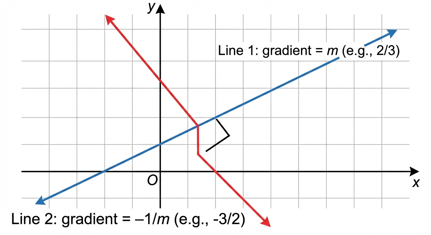
This rule is crucial for problems involving shapes like squares and rectangles, or finding altitudes and perpendicular bisectors, which are common exam favourites.
Worked example
Worked Example: Equation of a Perpendicular Bisector
Let's Slay This Classic Exam Question! 🚀
The coordinates of two points A and B are (2, 5) and (8, -1) respectively. Find the equation of the perpendicular bisector of the line segment AB, giving your answer in the form .
- 1Find the midpoint of AB. A 'bisector' cuts the line segment exactly in half, so we need the coordinates of this halfway point. We'll call it M.
- 2Calculate the gradient of the line segment AB. We need this to figure out the gradient of the line perpendicular to it.
- 3Determine the perpendicular gradient. Remember the rule: . Our perpendicular bisector's gradient () will be the negative reciprocal of .
- 4Construct the equation of the perpendicular bisector. We have everything we need! We have a point on the line (the midpoint M(5, 2)) and we have the gradient (). Let's plug these into our go-to formula: .
- 5Rearrange the equation into the required form . Examiners are picky about the final format, so always double-check the question!
Answer
3. Equations of Circles: Standard and General Forms
Alright, let's break down the equation of a circle. At its core, a circle is just a collection of points that are all the exact same distance from a central point. Think of it like a Wi-Fi signal – everyone within the radius gets the connection! This simple idea gives us the standard form of the equation, which is your new best friend: This formula is basically Pythagoras' theorem in disguise. The point is the centre of your circle, and is the radius. Super important: notice the minus signs in the brackets! This means if you see , the x-coordinate of the centre is , not . It's a classic trip-up, so watch out.
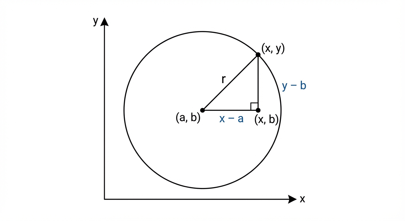
Now, examiners love to be tricky, so they often give you the equation in a messy, expanded form like . Your mission, should you choose to accept it, is to wrestle this beast back into the friendly standard form. The tool for this job? Completing the square, a skill you've already mastered from quadratics. By completing the square for both the x-terms and the y-terms, you can reveal the circle's true centre and radius. Mastering this conversion is non-negotiable for your exams and is fundamental for further studies in fields like engineering or computer graphics, where defining circular paths and boundaries is an everyday task.
Worked example
Finding the Centre and Radius from the General Form
Taming the Beast: From Chaos to Circle! 🦁
A circle C has the equation . Find the coordinates of the centre of C and the radius of C.
- 1First, let's rearrange the equation to group the x-terms and y-terms together, and move the constant to the other side. This sets the stage for completing the square.
- 2Now, complete the square for the x-terms. We take the coefficient of (which is -8), halve it (-4), and square it (16). We add this value to both sides of the equation to keep it balanced.
- 3Next, do the same for the y-terms. The coefficient of is 12. Halve it (6) and square it (36). Add this to both sides as well.
- 4The beauty of completing the square is that our grouped terms are now perfect squares. Let's factorise them into the and format and simplify the right-hand side.
- 5We've successfully converted to standard form! Now we can just read off the centre and the radius . Remember to be careful with the signs for the centre and to take the square root of the right side for the radius.
Answer
4. Intersection of Lines and Circles
Alright, let's tackle what happens when a straight line meets a circle. Think of it as solving a mystery: do they meet, and if so, where? Algebraically, this is a classic case of simultaneous equations. You'll have one linear equation for the line (e.g., ) and one quadratic for the circle (e.g., ). The game plan is to substitute the linear equation into the circle's equation. This clever move eliminates one variable, leaving you with a single, powerful quadratic equation in terms of either or .
Now, here's the pro-move that separates the experts from the novices: using the discriminant (). Before you even bother solving the quadratic, the discriminant tells you the whole story of their relationship.
Now, here's the pro-move that separates the experts from the novices: using the discriminant (). Before you even bother solving the quadratic, the discriminant tells you the whole story of their relationship.
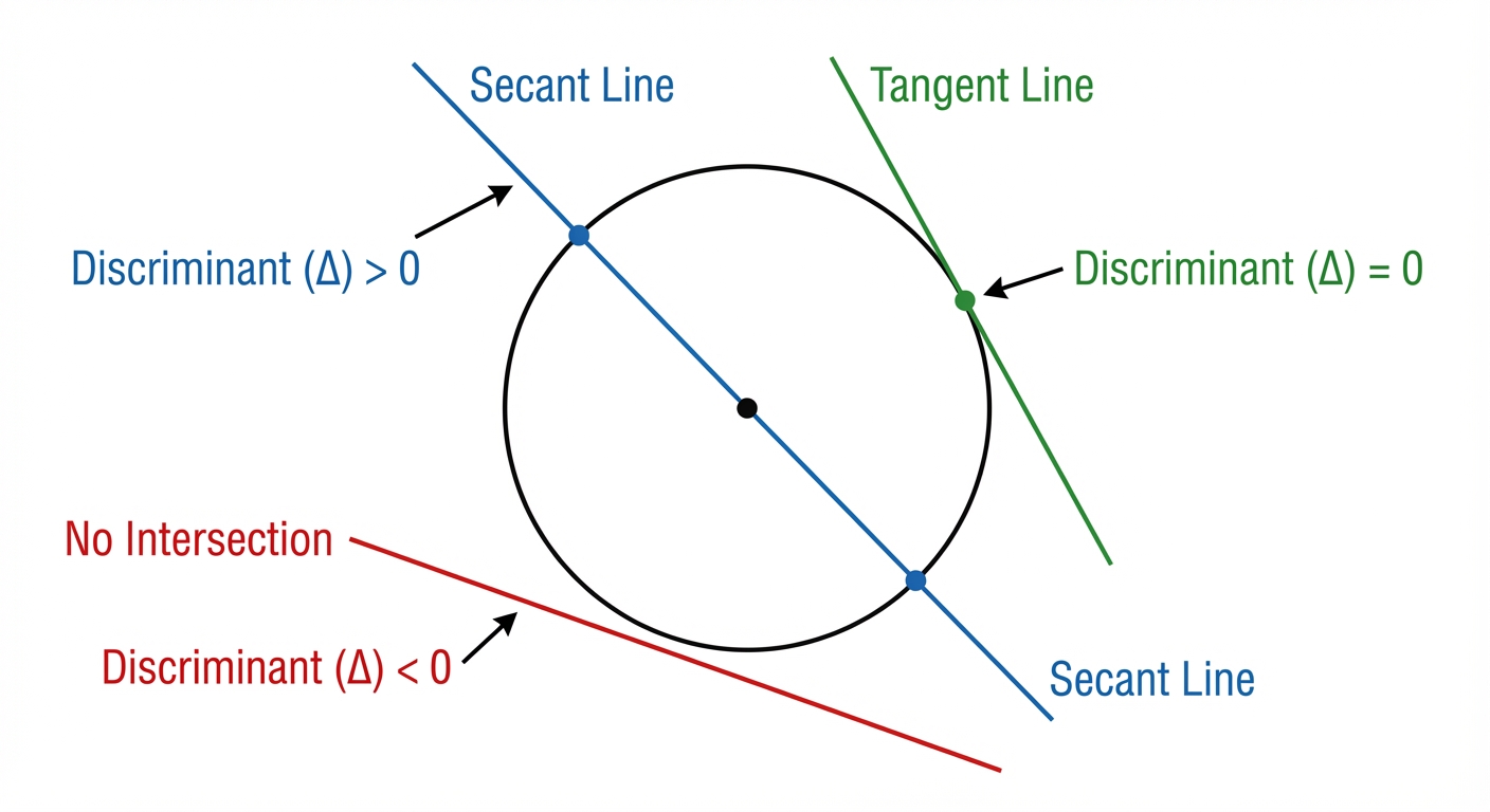
Here’s the breakdown:
• If , you get two distinct real roots. The line is a secant, cutting straight through the circle at two different points.
• If , there are no real roots. The line and circle completely miss each other. No drama, no intersection.
• The golden ticket: If , you have exactly one repeated real root. This is the condition for tangency – the line just grazes the circle at a single point. Mastering this is crucial for exams and foundational for university-level calculus and physics, where tangents describe rates of change and instantaneous velocity.
Worked example
Worked Example: Proving Tangency and Finding the Point of Contact
Let's Get This Bread 🍞
Show that the line is a tangent to the circle , and find the coordinates of the point of contact.
- 1First, we substitute the line equation into the circle equation. This combines them into a single equation in terms of , which we can then solve.
- 2Now, expand the brackets and rearrange everything to get a standard quadratic equation in the form . Make sure one side is zero!
- 3To show it's a tangent, we must prove there's only one point of intersection. We use the discriminant, . If it equals zero, we've proven tangency.
- 4Since the discriminant is 0, the line is a tangent. Now we solve our simplified quadratic to find the single x-coordinate of contact. You can factorise or use the quadratic formula.
- 5We're almost there! Substitute this x-value back into the easiest equation (the line equation!) to find the corresponding y-coordinate. Then, state your final answer clearly.
Answer
5. Intersection Conditions and the Discriminant
Alright, let's talk about one of the most powerful tools in your coordinate geometry arsenal: the discriminant. You already know that to find where two graphs intersect, you solve their equations simultaneously. But what if you don't need the exact points? What if you just need to know how many times they intersect? This is crucial for university-level problem-solving and a frequent A-Level exam question style.
When you set a linear equation (like ) equal to a quadratic curve (like ), you'll rearrange it into a new quadratic equation of the form . The roots of this specific quadratic are the x-coordinates of the points of intersection. Now, instead of fully solving it, we can use the discriminant, , to predict the outcome. It's like checking the movie trailer instead of watching the whole film.
Here's the breakdown:
1. Two Intersections (): If the discriminant is positive, we get two distinct real roots. This means the line cuts through the curve at two separate points. The line is called a secant.
2. One Intersection (): If the discriminant is zero, we get exactly one repeated real root. This is the special case where the line just touches the curve at a single point without crossing it. The line is a tangent to the curve. This condition is a superstar in exam questions! ⭐
3. No Intersections (): If the discriminant is negative, there are no real roots. The line and the curve completely miss each other, like two ships in the night.
When you set a linear equation (like ) equal to a quadratic curve (like ), you'll rearrange it into a new quadratic equation of the form . The roots of this specific quadratic are the x-coordinates of the points of intersection. Now, instead of fully solving it, we can use the discriminant, , to predict the outcome. It's like checking the movie trailer instead of watching the whole film.
Here's the breakdown:
1. Two Intersections (): If the discriminant is positive, we get two distinct real roots. This means the line cuts through the curve at two separate points. The line is called a secant.
2. One Intersection (): If the discriminant is zero, we get exactly one repeated real root. This is the special case where the line just touches the curve at a single point without crossing it. The line is a tangent to the curve. This condition is a superstar in exam questions! ⭐
3. No Intersections (): If the discriminant is negative, there are no real roots. The line and the curve completely miss each other, like two ships in the night.
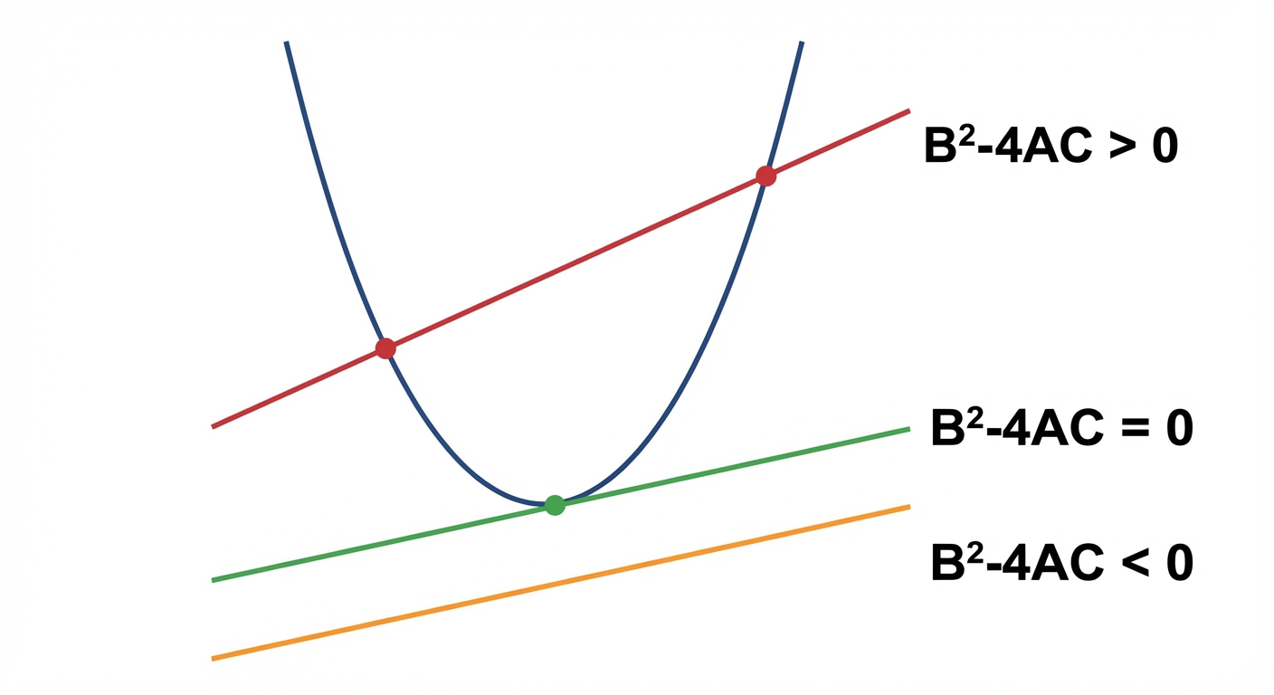
Often, you'll be given an equation with an unknown constant, say '', and asked to find the set of values of k for which a certain condition (e.g., tangency) is met. This is a classic application that tests your ability to form the quadratic, apply the correct discriminant condition, and solve the resulting inequality. Mastering this isn't just about passing P1; it's a foundational skill for understanding parameterisation in further maths and engineering.
Worked example
Worked Example: Finding a Set of Values for Two Distinct Intersections
Let's Find 'k' and Save the Day! ✨
Find the set of values of the constant for which the line intersects the curve at two distinct points.
- 1First things first, we need to find where the graphs could intersect. We do this by setting the two equations equal to each other. This combines them into a single equation that represents the intersection points.
- 2Now, we need to get this into the standard quadratic form . This is a non-negotiable step! Be super careful when collecting the terms, especially the terms which both involve variables and the constant .
- 3With our equation in standard form, we can clearly identify our coefficients , , and . Remember, '' is the entire coefficient of the term, including the negative sign and the bracket.
- 4The question asks for two distinct points, which is our cue to use the discriminant condition . We'll substitute our expressions for , , and into this inequality.
- 5We now have a quadratic inequality to solve for . Expand the bracket and simplify. To solve the inequality, find the 'critical values' by treating it as an equation ().
- 6The critical values are and . Since the inequality is 'greater than 0', we want the regions outside the roots of the parabola . A quick sketch helps visualize this. Therefore, the solution is the set of values where is less than the smaller root or greater than the larger root. ✅
Answer
Practice this in the app
Unlock the full chapter: practice questions, flashcards, mock papers and notes, free.
Continue revising