Chapter S2: The Poisson Distribution and its Approximations
Mastering Rare Events: From Poisson to Normal 🎲
Introduction
1. Introduction
Ever wondered about the probability of receiving a certain number of texts in an hour, or the number of shooting stars you might see on a clear night? Welcome to the Poisson distribution, our go-to tool for modelling random, rare events happening over a fixed interval of time or space! In this chapter, we're going to dive deep into this fascinating topic. First, we'll get to grips with calculating basic Poisson probabilities. Then, we'll see what happens when we combine two Poisson distributions (spoiler: it's surprisingly simple!). Next, we'll learn a super useful trick: how to use the Poisson distribution as a clever shortcut for the Binomial distribution when certain conditions are met. And finally, for when our numbers get really big, we'll explore how to approximate the Poisson distribution using the mighty Normal distribution. Let's get started! 💪
2. Calculating Probabilities using the Poisson Distribution
Alright, let's dive into the Poisson distribution. Think of it as the go-to model for events that are random and happen over a set interval of time or space. It’s like counting how many times a specific song comes up on your shuffled playlist per day. For this to work, a few conditions have to be met. First, events must be independent – getting one notification doesn't make another one more or less likely. Second, they must happen at a constant average rate. If you get an average of 10 DMs per hour, that rate () should be steady. Finally, events can't happen at the exact same time.
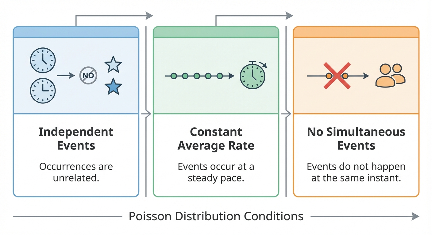
The star of the show is the parameter (lambda). It’s the mean number of events in the given interval, so . The super cool and unique thing about Poisson is that the variance is also equal to lambda! So, . This is a key property to remember. Once you know your scenario fits a Poisson model, you can use its probability formula to find the chance of an event happening a specific number of times. The formula is: Here, is the exact number of events you’re interested in. So, if we know the average number of interruptions from your family while gaming is per hour, we can use this formula to find the probability of getting exactly interruptions in the next hour. It’s your key to predicting the unpredictable!
Worked example
Worked Example: Calculating a Specific Poisson Probability
Spam Calls & Probability 📞
A student receives spam calls at an average rate of 2.5 per day. Assuming the number of calls received per day follows a Poisson distribution, calculate the probability that they receive exactly 3 spam calls tomorrow.
- 1First, we need to define our random variable and its distribution. Let be the number of spam calls received in a day. The problem states this follows a Poisson distribution with an average rate of 2.5. So, our mean is 2.5. We write this as:
- 2We want to find the probability of receiving exactly 3 calls, so our target value is . Now, let's write down the Poisson probability formula we're going to use.
- 3Time to substitute our values into the formula. We'll plug in and .
- 4Now, grab your calculator and compute the value. Remember that .
- 5Finally, state your answer clearly. The probability of the student receiving exactly 3 spam calls tomorrow is about 0.214 (to 3 s.f.). So, roughly a 21.4% chance. Not bad!
Answer
3. The Sum of Independent Poisson Distributions
Alright, let's talk about one of the coolest and most straightforward rules in S2. Imagine you're tracking two different things that happen randomly but at a steady average rate. For example, the number of DMs you get on Insta in an hour, let's call that , and the number of Snaps you get, let's call that . If these two things are independent (getting a Snap doesn't make you more or less likely to get an Insta DM), and they both follow a Poisson distribution, we can do something awesome.
The core idea is this: If and are independent random variables, then their sum, , also follows a Poisson distribution. And the best part? The new rate is just the sum of the old rates! So, . It's that simple. You literally just add the lambdas together. This is a massive shortcut. Instead of dealing with two separate distributions, you can combine them into one super-distribution for the total number of events.
The core idea is this: If and are independent random variables, then their sum, , also follows a Poisson distribution. And the best part? The new rate is just the sum of the old rates! So, . It's that simple. You literally just add the lambdas together. This is a massive shortcut. Instead of dealing with two separate distributions, you can combine them into one super-distribution for the total number of events.
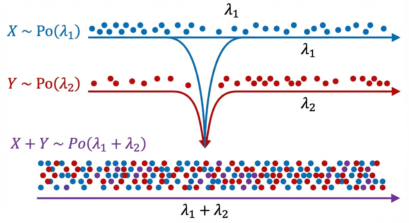
The keyword here, and don't you forget it, is independent. This rule only works if the two variables don't influence each other. Think of it like two different artists on Spotify; the number of times you stream Artist A doesn't affect the number of times you stream Artist B. But if you were looking at the number of goals from your favourite striker and the total number of goals for their team, those are not independent, so you couldn't use this rule. For any A-Level question, they'll usually tell you to assume independence, but it's a critical concept to have locked down. So next time you see two independent Poisson variables, you know what to do: combine forces and add those lambdas! 🚀
Worked example
Worked Example: Drive-Thru Orders
Serving Up Some Poisson Sums 🍔
At a fast-food drive-thru between 5 PM and 6 PM, the number of customers ordering burgers, , follows a Poisson distribution with a mean of 8.2. The number of customers ordering just drinks, , follows an independent Poisson distribution with a mean of 4.6.
a) Find the probability that exactly 15 customers come through the drive-thru in this hour.
b) Find the probability that fewer than 10 customers come through the drive-thru in this hour.
a) Find the probability that exactly 15 customers come through the drive-thru in this hour.
b) Find the probability that fewer than 10 customers come through the drive-thru in this hour.
- 1First, we need to define a new variable for the total number of customers. Let's call it . Since ordering a burger and ordering a drink are independent events, we can find the distribution for by adding the two individual Poisson distributions together.
- 2Now, we apply the sum rule. We know and . We just add the lambdas to find the distribution for .
- 3For part (a), we need to find the probability that exactly 15 customers arrive, which is . We use the Poisson probability formula: .
- 4For part (b), we need the probability of fewer than 10 customers. This means , which is the same as . We have to sum the probabilities for . In an exam, you'd use the cumulative tables for this, but the calculation represents this sum.
- 5Using the cumulative Poisson distribution tables (or a calculator), we look up the value for and . This gives us the final answer for part (b).
Answer
4. The Poisson Approximation to the Binomial Distribution
Okay, let's be real. Sometimes the Binomial distribution is just... extra. Imagine you're checking the number of typos in a 10,000-word essay. The number of words, , is huge, but the probability, , of any single word having a typo is tiny. Trying to calculate using the Binomial formula would be a nightmare. We're talking massive factorials and tiny probabilities that would make your calculator cry. 🤯
This is where the Poisson distribution slides into the DMs as the perfect approximation. It's like a brilliant cheat code for a specific gaming scenario. We can swap out the complicated Binomial for a much simpler Poisson if two conditions are met:
1. is large: The number of trials needs to be big. The general rule of thumb is .
2. is small: The probability of success on any one trial needs to be tiny.
Crucially, the product of these two, , must be small (usually ). This product, , is the VIP of this whole operation. It becomes the mean of our new Poisson distribution, . So, if you have a random variable and it meets the conditions, you can approximate it with a new variable , where .
This is where the Poisson distribution slides into the DMs as the perfect approximation. It's like a brilliant cheat code for a specific gaming scenario. We can swap out the complicated Binomial for a much simpler Poisson if two conditions are met:
1. is large: The number of trials needs to be big. The general rule of thumb is .
2. is small: The probability of success on any one trial needs to be tiny.
Crucially, the product of these two, , must be small (usually ). This product, , is the VIP of this whole operation. It becomes the mean of our new Poisson distribution, . So, if you have a random variable and it meets the conditions, you can approximate it with a new variable , where .
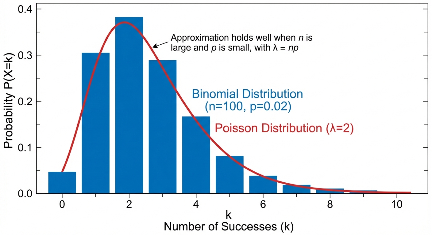
This trick saves a ton of calculation time and is super useful for modelling rare events over a large number of opportunities, like finding a rare Pokémon in a huge area or the number of faulty phone screens in a massive factory shipment.
Worked example
Worked Example: Approximating Faulty Components
Dodgy Airpods in a Massive Shipment 🎧
A company manufactures wireless earbuds. It is known that on average, 1 in every 800 earbuds is faulty. In a large shipment of 2400 earbuds, find the probability that there are fewer than 3 faulty ones.
- 1First, let's define our Binomial distribution and check if we can even use the Poisson approximation. We need to see if is large () and is small ().Let be the number of faulty earbuds.
(the total number of earbuds)
(the probability of one being faulty)
Checking the conditions:
✅
✅
Since both conditions are met, we can use a Poisson approximation. - 2Now we can define our new Poisson distribution. The mean, , is just the value of we just calculated. This is the parameter for our new distribution, let's call it .
So, we can approximate with . - 3The question asks for the probability of 'fewer than 3' faulty earbuds. This means we need to find . Remember, 'fewer than 3' doesn't include 3, so we're looking for the sum of probabilities for , , and .
- 4Time to plug the values into the Poisson formula, , for each case and add them up. Let's get that calculator ready!
So, the probability is approximately 0.423 (to 3 s.f.).
Answer
So, the probability is approximately 0.423 (to 3 s.f.).
So, the probability is approximately 0.423 (to 3 s.f.).
5. The Normal Approximation to the Poisson Distribution
Alright, so you've mastered the Poisson distribution for things that happen randomly over time or space, like getting DMs or finding rare items in a game. But what happens when the numbers get huge? Calculating Poisson probabilities when the mean, , is massive (like, say, the number of views on a viral TikTok in an hour) is a total nightmare. The factorials get ridiculously big and your calculator will just give up. 💀
This is where the Normal distribution swoops in to save the day! When is large enough (the magic number is usually ), the shape of the Poisson distribution starts to look a lot like the classic bell curve of the Normal distribution. So, we can use the Normal distribution as a super-close approximation. If a variable follows a Poisson distribution, , we can approximate it with a Normal distribution, . The best part? The mean and variance are the same! So, and .
But there's one critical catch. Poisson is discrete (you can get 20 likes, but not 20.5), while Normal is continuous. It's like the difference between skipping through songs on Spotify (discrete tracks) versus smoothly sliding the progress bar (continuous time). To bridge this gap, we use something called continuity correction. We have to adjust our discrete value by 0.5 to properly capture the area under the continuous curve.
This is where the Normal distribution swoops in to save the day! When is large enough (the magic number is usually ), the shape of the Poisson distribution starts to look a lot like the classic bell curve of the Normal distribution. So, we can use the Normal distribution as a super-close approximation. If a variable follows a Poisson distribution, , we can approximate it with a Normal distribution, . The best part? The mean and variance are the same! So, and .
But there's one critical catch. Poisson is discrete (you can get 20 likes, but not 20.5), while Normal is continuous. It's like the difference between skipping through songs on Spotify (discrete tracks) versus smoothly sliding the progress bar (continuous time). To bridge this gap, we use something called continuity correction. We have to adjust our discrete value by 0.5 to properly capture the area under the continuous curve.
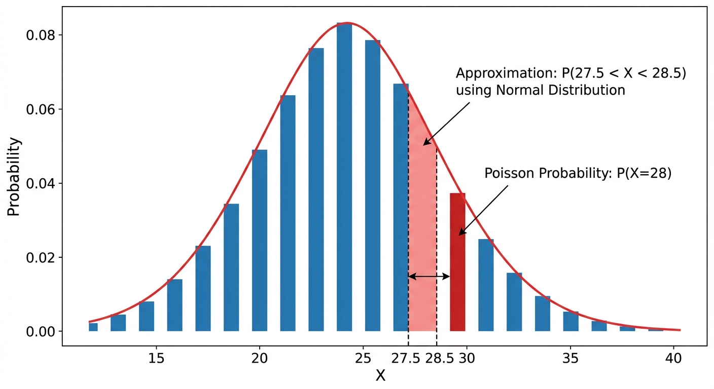
For example, to find , we'd look for the area between 19.5 and 20.5 on our Normal curve. To find , we'd look for the area above 20.5. Once you've applied the continuity correction, you just standardise using and find the probability like a regular Normal distribution problem. Easy peasy.
Worked example
Worked Example: Applying the Normal Approximation
Calculating Server Traffic 💻
The number of messages posted in a popular Discord server's #memes channel follows a Poisson distribution with a mean of 60 messages per minute. Find the probability that in a given minute, fewer than 55 messages are posted.
- 1First, let's define our variable and check if we can even use the Normal approximation. We need to be greater than 15.Let be the number of messages per minute.
.
Since , and , the Normal approximation is appropriate. - 2Now, we define the Normal distribution we'll use for the approximation. Remember, the mean and variance are both equal to .
So, our mean is and our variance is . - 3Here comes the crucial part: continuity correction. We want to find the probability of fewer than 55 messages (). Since must be an integer, this is the same as . For our continuous variable , we need to include the entire 'bar' for 54, so we go up to 54.5.
- 4Time to standardise! We convert our value into a -score using the standard formula so we can use the Normal distribution tables.
- 5Finally, we find the probability using the -score. We're looking for . Since the value is negative, we use the symmetry of the Normal curve.
From the tables, .
So, . - 6And we're done! Let's write down the final answer, rounded to 3 significant figures as is standard practice.The probability of fewer than 55 messages being posted is 0.239 (3 s.f.).
Answer
The probability of fewer than 55 messages being posted is 0.239 (3 s.f.).
Practice this in the app
Unlock the full chapter: practice questions, flashcards, mock papers and notes, free.
Continue revising