S2: Sampling and Estimation
Making Smart Guesses About The World 🌍
Introduction
1. Introduction
Ever wondered how companies know the average opinion of millions of customers without asking everyone? Or how scientists can estimate the average size of a fish in a huge lake? That's the magic of sampling! In this chapter, we're diving into the powerful techniques statisticians use to learn about a massive group (a population) by studying a small, manageable part of it (a sample). First, we'll figure out how to make our sample's statistics a fair and unbiased estimate of the whole population's values. Then, we'll explore the super-important Central Limit Theorem to understand the distribution of the sample mean – it’s a game-changer! Finally, we'll learn how to build confidence intervals, which give us a range of values where we can be pretty sure the true population mean lies. Let's get ready to turn small clues into big conclusions! 🕵️♀️
2. Unbiased Estimates of Population Parameters
Okay, let's get into it. Imagine you're trying to figure out the true average listening time on Spotify for all students in your year group. That true average is the population mean, which we call . Obviously, you can't survey everyone. So, you grab a sample – say, 10 of your friends – and find their average listening time. This is your sample mean, . Now, the big question is: how good is your sample mean as a guess for the real population mean? This is where the idea of an unbiased estimate comes in. An estimator is unbiased if it doesn't systematically over- or under-shoot the target. Think of it like an aim assist in a game that's perfectly calibrated. A good, unbiased estimator might not be perfect every time, but its average shot is right on target. Your sample mean, , is a perfect, unbiased estimator for the population mean . It's your best shot, and on average, it's spot on. Easy!
But what about the variance of listening times, ? This is where it gets a little more complex. If you just calculate the variance of your sample of 10 friends and divide by , you'll actually end up with a value that's, on average, too small. This is a biased estimate! Why? Because your friends' listening times are naturally going to be closer to their own little group average () than they are to the true average of the entire year group (). To correct for this sneaky underestimation, we have to adjust our formula.
But what about the variance of listening times, ? This is where it gets a little more complex. If you just calculate the variance of your sample of 10 friends and divide by , you'll actually end up with a value that's, on average, too small. This is a biased estimate! Why? Because your friends' listening times are naturally going to be closer to their own little group average () than they are to the true average of the entire year group (). To correct for this sneaky underestimation, we have to adjust our formula.
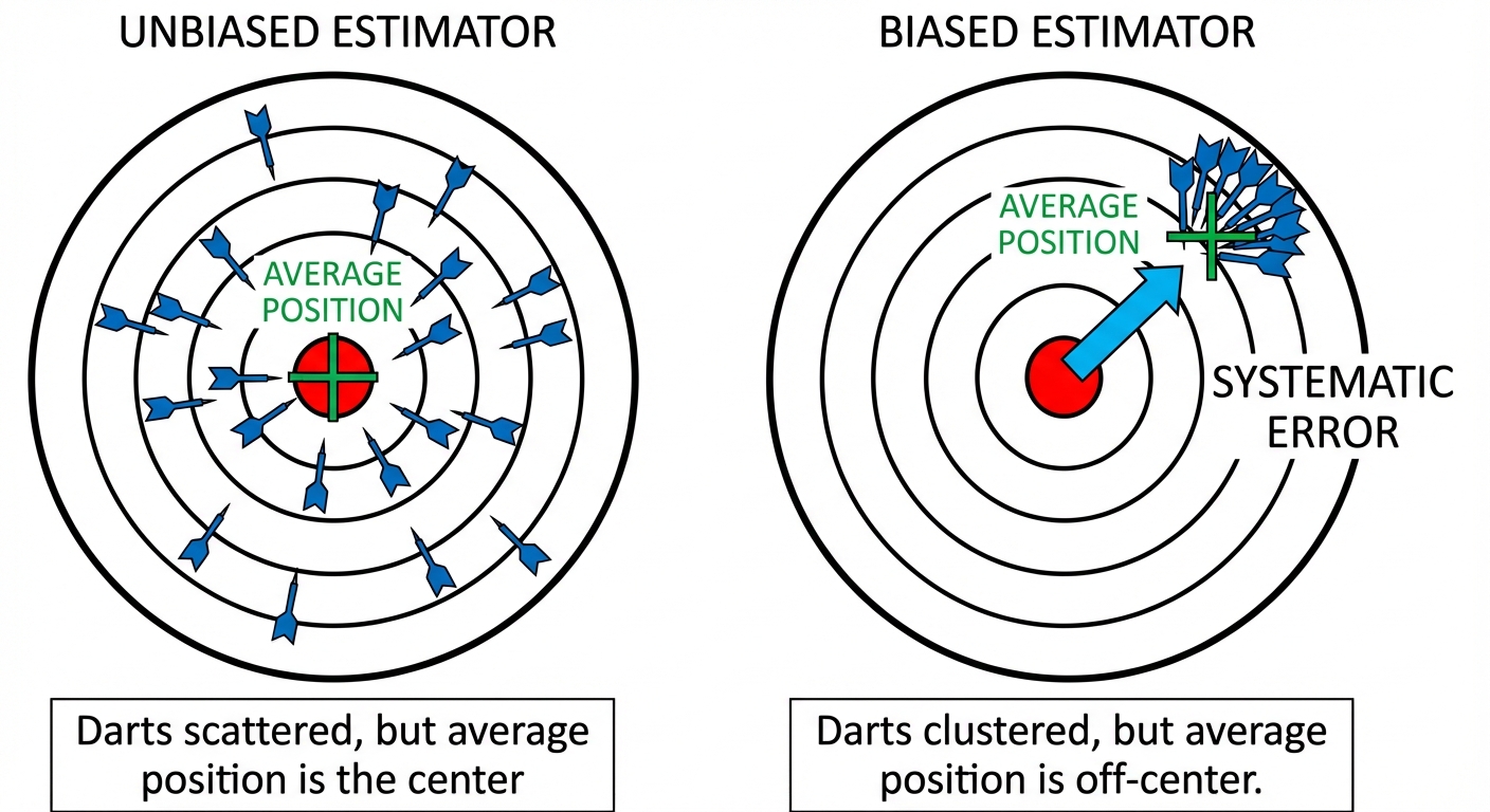
We create an unbiased estimate of the population variance, which we call , by dividing by instead of . This makes our result a little bit bigger, perfectly counteracting the bias. It's the ultimate stats hack.
So, for any sample of size , the two key estimates you need are:
Unbiased estimate of population mean ():
Unbiased estimate of population variance ():
So, for any sample of size , the two key estimates you need are:
Unbiased estimate of population mean ():
Unbiased estimate of population variance ():
Worked example
Calculating Unbiased Estimates from Sample Data
Let's Crunch Some Numbers 💻
You track the number of hours you worked at your part-time barista job over a random sample of 6 days. The hours are: 5, 8, 4, 7, 5, 9. Calculate unbiased estimates for the mean and variance of the number of hours you work per day.
- 1First, let's find the sample mean, . This is our unbiased estimate for the true mean number of hours, . We just add up the hours and divide by the number of days, .
- 2Next, we need the ingredients for our variance formula, . We already have and . Now we need to find the sum of the squares, .
- 3Time to plug everything into the magic formula for the unbiased estimate of variance. The key is to divide by , which is .
- 4Finally, state your answers clearly. We've found the unbiased estimates for the population mean and variance based on your sample data.Unbiased estimate of population mean is .
Unbiased estimate of population variance is .
Answer
Unbiased estimate of population mean is .
Unbiased estimate of population variance is .
Unbiased estimate of population variance is .
3. The Distribution of the Sample Mean
Okay, let's get real. Imagine you want to find the average amount of time students at your school spend on Spotify each day. Asking every single person is impossible, right? That's the population. Instead, you grab a sample, say 50 friends, and find their average time. This average is your sample mean, which we call .
Now, what if your friend also took a sample of 50 different people? Their sample mean would probably be slightly different from yours. If we took tons of these samples and plotted all their means, we'd get a new distribution: the distribution of the sample mean. So, what are its properties?
First, the average of all these sample means will be the true average of the whole school. Makes sense, right? So, the expected value of the sample mean is just the population mean: .
Second, the spread of the sample means will be smaller than the spread of the individual times. Think about it: getting a sample where everyone listens for 10 hours is super unlikely compared to finding one person who does. The bigger your sample size (), the more the sample means will 'huddle' around the true mean. The variance is given by , where is the population variance.
Now, what if your friend also took a sample of 50 different people? Their sample mean would probably be slightly different from yours. If we took tons of these samples and plotted all their means, we'd get a new distribution: the distribution of the sample mean. So, what are its properties?
First, the average of all these sample means will be the true average of the whole school. Makes sense, right? So, the expected value of the sample mean is just the population mean: .
Second, the spread of the sample means will be smaller than the spread of the individual times. Think about it: getting a sample where everyone listens for 10 hours is super unlikely compared to finding one person who does. The bigger your sample size (), the more the sample means will 'huddle' around the true mean. The variance is given by , where is the population variance.
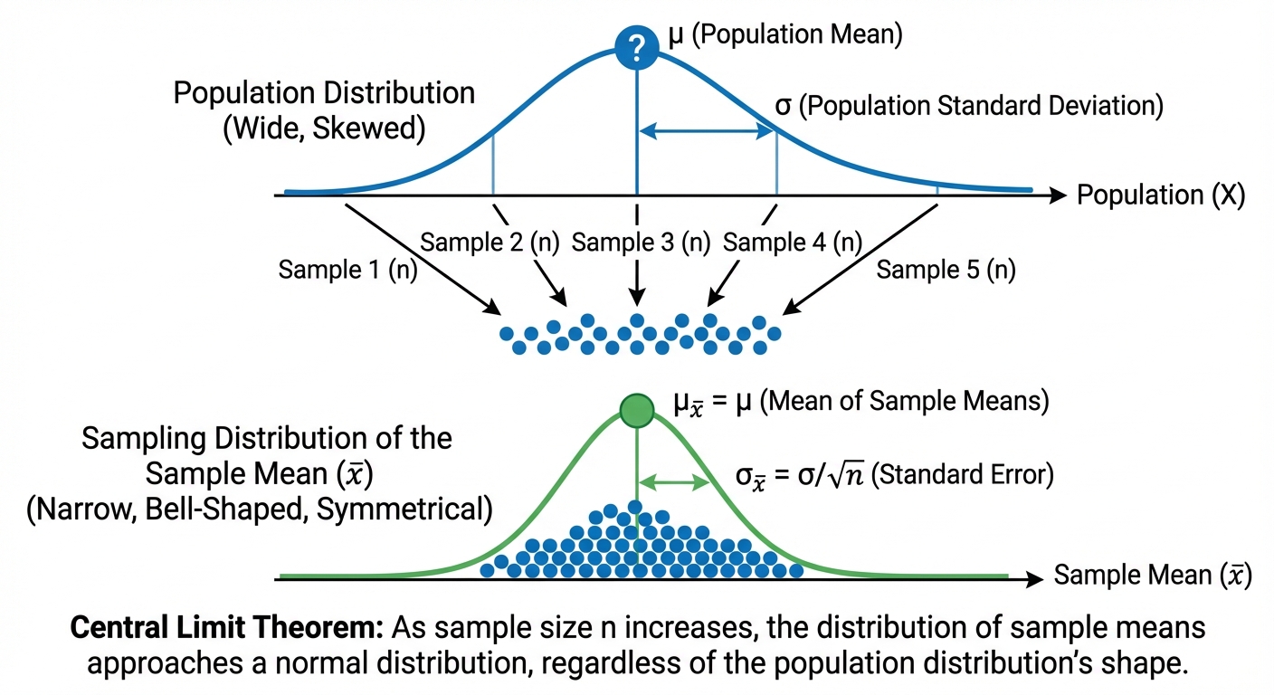
This leads us to the MVP of statistics: the Central Limit Theorem (CLT). This is a total game-changer. The CLT states that if your sample size () is large enough (usually ), the distribution of the sample mean will be approximately a Normal distribution, even if the original population wasn't Normal at all. It's like putting a weirdly shaped playlist on shuffle and discovering it creates a perfectly balanced vibe. This is clutch because it lets us use our Z-scores and Normal distribution tables to find probabilities about the sample mean, which is incredibly powerful.
Worked example
Worked Example: Applying the Central Limit Theorem
Let's See This in Action 🎮
The time, in minutes, that a student spends on a part-time weekend job has a mean of 480 minutes and a standard deviation of 60 minutes. The distribution of these times is unknown. A random sample of 35 students is taken. Find the probability that the mean time spent working for this sample is more than 500 minutes.
- 1First, let's pull out all the key info from the problem. We're given the population mean (), population standard deviation (), and our sample size ().
- 2The original distribution is unknown, but our sample size is greater than 30. This is our green light to use the Central Limit Theorem! This means we can treat the distribution of the sample mean, , as a Normal distribution.
- 3Now, let's define the parameters for the distribution of . The mean of is just , and its variance is .
- 4We need to find . To do this, we standardize the value 500 to find its Z-score. Remember the formula: .
- 5Now we look up this Z-score in our standard normal distribution tables or use a calculator. We want the area to the right of our Z-score, since the question asks for 'more than' 500 minutes.
- 6Finally, write down the answer. So, there's about a 2.43% chance that the average work time for a sample of 35 students will be over 500 minutes. Not very likely, but totally possible!
Answer
4. Confidence Intervals for Population Mean and Proportion
Okay, so imagine you want to know the true average time students at your school spend on TikTok. Asking every single person is impossible, right? So you take a sample, say 50 people, and find their average. This sample mean, , is a good point estimate, but it's probably not the exact true mean, . It's like trying to guess a song's BPM by tapping for 10 seconds—you'll be close, but not perfect.
This is where Confidence Intervals (CIs) come in. A CI is a range of values where we're pretty confident the true population parameter (like the mean or proportion ) actually lives. Instead of saying "the average is 2.1 hours", we say "we're 95% confident the average is between 1.9 and 2.3 hours." This range gives us a margin for error.
The formula for a CI for the mean (when we know the population variance ) is:
And for a proportion:
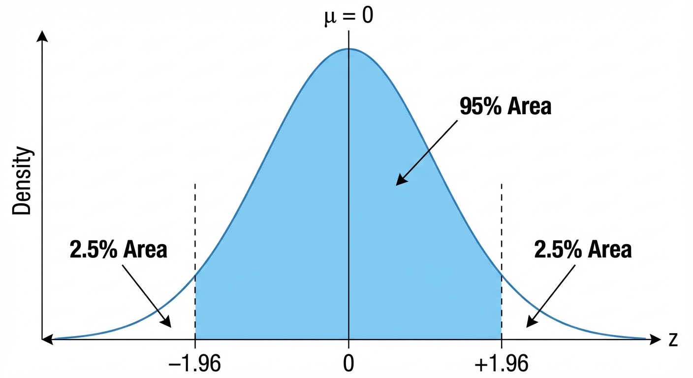
The 'z' value, or z-critical value, is the secret sauce. It's determined by your chosen confidence level (usually 90%, 95%, or 99%). For a 95% confidence level, the z-value is always 1.96. This number comes from the standard normal distribution and basically tells us how many standard deviations away from the mean we need to go to capture 95% of the possibilities.
This is where Confidence Intervals (CIs) come in. A CI is a range of values where we're pretty confident the true population parameter (like the mean or proportion ) actually lives. Instead of saying "the average is 2.1 hours", we say "we're 95% confident the average is between 1.9 and 2.3 hours." This range gives us a margin for error.
The formula for a CI for the mean (when we know the population variance ) is:
And for a proportion:
The 'z' value, or z-critical value, is the secret sauce. It's determined by your chosen confidence level (usually 90%, 95%, or 99%). For a 95% confidence level, the z-value is always 1.96. This number comes from the standard normal distribution and basically tells us how many standard deviations away from the mean we need to go to capture 95% of the possibilities.
Thinking about sample size, ? If you want a more precise, narrower interval (like estimating your exam score to be between 88-90% instead of 80-98%), you'll need a larger sample size. More data means more confidence and less uncertainty. It's like having more reviews before buying a new game—you get a much better idea of its true quality.
Worked example
Worked Example: Confidence Interval for a Population Proportion
What's the Real Tea on Part-Time Jobs? 💼
A researcher wants to estimate the proportion of A-Level students who have a part-time job. They survey a random sample of 250 students and find that 95 of them have a part-time job. Calculate a 99% confidence interval for the true proportion of all A-Level students with a part-time job.
- 1First, let's figure out our sample proportion () and find the correct z-value. The sample proportion is just the number of students with jobs divided by the total sample size. For a 99% confidence level, the z-value is a standard value you should memorize.
For 99% confidence, - 2Now, we need to calculate the margin of error (the part we add and subtract). This is the 'wiggle room' around our sample proportion. We'll use the formula for the standard error of a proportion and multiply by our z-value.
- 3Let's plug in our numbers: , , and . Be careful with the calculation under the square root!
- 4Finally, we build the interval by taking our sample proportion and adding/subtracting the margin of error we just found. This will give us our lower and upper bounds.
- 5Let's state our final answer clearly as an interval and write a concluding sentence to explain what it means in the context of the problem. This shows you understand the result.
So, the 99% CI is (0.301, 0.459). We are 99% confident that the true proportion of all A-Level students with a part-time job is between 30.1% and 45.9%.
Answer
So, the 99% CI is (0.301, 0.459). We are 99% confident that the true proportion of all A-Level students with a part-time job is between 30.1% and 45.9%.
So, the 99% CI is (0.301, 0.459). We are 99% confident that the true proportion of all A-Level students with a part-time job is between 30.1% and 45.9%.
Practice this in the app
Unlock the full chapter: practice questions, flashcards, mock papers and notes, free.
Continue revising