S1 Chapter 5: The Normal Distribution
Mastering the Famous Bell Curve! 🔔
Introduction
1. Introduction
Alright, let's dive into one of the most important and frequently seen distributions in statistics: the Normal Distribution. You've probably seen its classic 'bell curve' shape everywhere, from test scores to heights. In this chapter, we're going to get super comfortable with it. First, we'll learn how to calculate probabilities – basically, finding the area under the curve for any given range. Then, we'll flip the problem on its head and tackle inverse problems, where you're given the probability and have to find the specific value. Finally, we'll uncover a powerful exam trick: using the Normal distribution as a clever approximation for the Binomial distribution when our numbers get really big. It's a game-changer, trust me. Let's get this done! 💪
2. Calculating Probabilities using the Standard Normal Distribution
Okay, so we know that tons of things in the real world follow a Normal Distribution, from IQ scores to the height of students in your year group. The catch is, each of these has its own unique mean () and standard deviation (). It would be a nightmare to have a separate probability table for every single possible combination of and ! This is where the hero of our story comes in: the Standard Normal Distribution, . Think of it as the 'master template' or the OG bell curve. It has a mean of 0 and a standard deviation of 1.
The magic trick we use is called standardisation. We convert any value, , from any normal distribution, , into a 'Z-score' using this powerhouse formula:
This Z-score literally tells you how many standard deviations your value is away from its mean . A positive Z means it's above the mean; a negative Z means it's below. Once you have this Z-score, you can use the standard normal probability tables (the table in your formula booklet) to find the required probability. This process allows us to solve problems for any normal distribution using just one table. It's incredibly efficient.
The magic trick we use is called standardisation. We convert any value, , from any normal distribution, , into a 'Z-score' using this powerhouse formula:
This Z-score literally tells you how many standard deviations your value is away from its mean . A positive Z means it's above the mean; a negative Z means it's below. Once you have this Z-score, you can use the standard normal probability tables (the table in your formula booklet) to find the required probability. This process allows us to solve problems for any normal distribution using just one table. It's incredibly efficient.
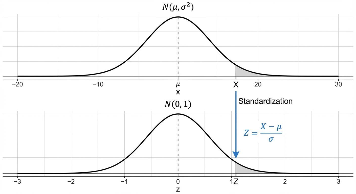
Pro-tip for exams and beyond: Always sketch the normal curve for the problem! Shade the area you're trying to find. This simple step is a game-changer for avoiding common errors, especially when calculating probabilities like (which requires ) or (which requires ). This skill is fundamental for university-level stats, finance, and data science, so mastering it now is a huge win. 💪
Worked example
Worked Example: Smartphone Battery Life Probability
Let's See This Standardisation Thing in Action 🎬
The battery life, hours, of a particular smartphone model is modelled by a normal distribution, . Find the probability that a randomly chosen smartphone of this model has a battery life of less than 20 hours.
- 1State the parameters and the required probability. We're given the distribution , so we have the mean and standard deviation . We need to find .
- 2Standardise the value to find its Z-score. This transforms our specific value into a value on the standard normal scale, allowing us to use the universal probability tables.
- 3Relate the original probability to the standardised probability and sketch the curve. Finding is equivalent to finding . A quick sketch shows we are looking for the area in the left tail of the standard normal distribution.P(X < 20) = P(Z < -1.6)
\text{[IMAGE_PLACEHOLDER_2: Sketch of the standard normal curve, mean at 0, with the area to the left of Z=-1.6 shaded.]} - 4Use the standard normal tables and the symmetry property. The tables provide for positive . For negative values, we use the rule . We look up in the table.
- 5Calculate the final probability and state the conclusion. The probability that a smartphone's battery lasts less than 20 hours is approximately 0.0548.
Answer
3. Inverse Normal Distribution Problems
Alright, so far we've been taking an x-value (like your score on a test) and finding the probability of getting it. Now, we're going to flip the script. Welcome to Inverse Normal Problems, where you're the stats detective 🕵️♀️. You're given the probability—the clue—and you have to find the specific value of , the mean , or the standard deviation .
Think of it like this: instead of your friend telling you they'll arrive in 20 minutes and you figuring out the chances they're late, they text you, "There's a 90% chance I'll be there by..." and you have to figure out the time. That's an inverse problem! The key move here is using the Standard Normal Distribution table in reverse. Instead of finding the z-score on the edges and looking for the probability in the middle, you'll find the given probability (or one close to it) in the main body of the table and then read outwards to find the corresponding z-score.
Think of it like this: instead of your friend telling you they'll arrive in 20 minutes and you figuring out the chances they're late, they text you, "There's a 90% chance I'll be there by..." and you have to figure out the time. That's an inverse problem! The key move here is using the Standard Normal Distribution table in reverse. Instead of finding the z-score on the edges and looking for the probability in the middle, you'll find the given probability (or one close to it) in the main body of the table and then read outwards to find the corresponding z-score.
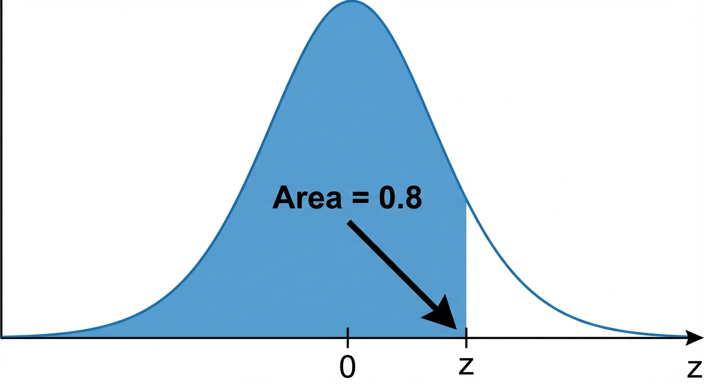
Remember, the table gives you the area to the left (). If you're given a 'greater than' probability, like the top 10% of students, you'll need to use symmetry. is the same as . You'd then look up 0.9000 in the table to find your z-score. Once you have that magic z-score, you just pop it into the standardisation formula, , and solve for whichever piece of the puzzle (, , or ) is missing. It's all about working backwards from the probability to the real-world value.
Worked example
Worked Example: Finding a Value Given a Probability
What Score Do You Need to Go Pro? 🎮
The time it takes for a group of players to complete a certain gaming level, minutes, is normally distributed with a mean of 40 minutes and a standard deviation of 5 minutes. The game developers want to invite the fastest 15% of players to a special tournament. What is the maximum time a player can take to complete the level to be invited?
- 1First, let's define our distribution. We're told the mean () and standard deviation (), so we can write down the normal distribution for the time .
- 2Now, let's turn the question into a probability statement. We're looking for the 'fastest 15%', which means the lowest 15% of times. We need to find a time, let's call it , where the probability of being less than or equal to it is 0.15.
- 3Time to standardize! We convert our variable into the standard normal variable . This lets us use the standard lookup table.
- 4Here's the inverse part. We need to find the z-score that corresponds to a probability of 0.15. Since our table gives probabilities greater than 0.5, we use symmetry. The z-score for 0.15 will be the negative of the z-score for . Looking up 0.85 in the table gives a z-score of approximately 1.036. So, our z-score is -1.036.
- 5Almost there! Now we set our standardized expression equal to the z-score we just found and solve for . This will give us the actual time in minutes.
- 6Finally, state the answer clearly in the context of the problem. A player needs to be pretty quick to get that invite!A player must complete the level in a maximum of 34.8 minutes (to 3 s.f.) to be invited to the tournament.
Answer
A player must complete the level in a maximum of 34.8 minutes (to 3 s.f.) to be invited to the tournament.
4. The Normal Approximation to the Binomial Distribution
Alright, let's talk about a major hack for when you're dealing with the Binomial distribution. You know how calculating binomial probabilities can be super tedious, especially when your number of trials, , is huge? Like, imagine trying to find the probability of exactly 70 out of 150 people preferring a certain brand of trainers. The calculation for is a nightmare. It's like trying to scroll to the very first message in a massive group chat – nobody has time for that. This is where the Normal distribution swoops in to save the day! If the sample size is big enough, the shape of the binomial distribution starts to look a lot like the classic bell curve of the normal distribution.
But hold up, you can't just use this approximation whenever you feel like it. There's a vibe check you have to pass first. The conditions are: and (where ). If both of these are true, you're good to go. If not, the approximation won't be accurate, and you'll have to stick with the old-school binomial method. When the conditions are met, we can approximate our binomial distribution with a normal distribution , where the mean is and the variance is .
Here's the crucial final step: the continuity correction. This sounds complicated, but it's just a way to handle the fact that we're using a continuous distribution (Normal) to model a discrete one (Binomial). Binomial deals with whole numbers (you can't have 4.5 successful free throws), while Normal can take any value. To bridge this gap, we adjust our discrete value by 0.5. Think of the binomial probabilities as rectangular bars on a histogram. To find the probability for a bar labelled 'k', we find the area under the normal curve from the left edge () to the right edge ().
But hold up, you can't just use this approximation whenever you feel like it. There's a vibe check you have to pass first. The conditions are: and (where ). If both of these are true, you're good to go. If not, the approximation won't be accurate, and you'll have to stick with the old-school binomial method. When the conditions are met, we can approximate our binomial distribution with a normal distribution , where the mean is and the variance is .
Here's the crucial final step: the continuity correction. This sounds complicated, but it's just a way to handle the fact that we're using a continuous distribution (Normal) to model a discrete one (Binomial). Binomial deals with whole numbers (you can't have 4.5 successful free throws), while Normal can take any value. To bridge this gap, we adjust our discrete value by 0.5. Think of the binomial probabilities as rectangular bars on a histogram. To find the probability for a bar labelled 'k', we find the area under the normal curve from the left edge () to the right edge ().
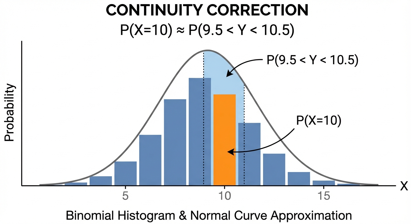
. So, for example, becomes , and becomes . Getting this right is the key to acing these questions! 🚀
Worked example
Worked Example: Approximating Probabilities for a Large Sample
Let's See This Hack in Action 🕵️
A popular new game is downloaded by a large number of people. It is known that 15% of players will purchase the 'premium pass'. A random sample of 200 players is taken. Find the probability that fewer than 25 players in the sample purchased the premium pass.
- 1First, let's define our binomial distribution and check if we can even use the normal approximation. We need to make sure and . Here, and .
- 2Now we can define our normal approximation. We need to calculate the mean () and the variance () for our new normal distribution, .
- 3The question asks for the probability of fewer than 25 players, which is . This means can be . For our continuous variable , we need to apply the continuity correction. 'Less than 25' means we include everything up to, but not including, 25. The corresponding continuous value is 24.5.
- 4Time to standardise! We convert our value of 24.5 into a Z-score so we can use the standard normal tables. Remember the formula . Don't forget to use the standard deviation, , which is the square root of the variance.
- 5Finally, we find the probability using the Z-score. We need to find . Since the Z-value is negative, we use the symmetry of the normal distribution: .
Answer
Practice this in the app
Unlock the full chapter: practice questions, flashcards, mock papers and notes, free.
Continue revising