Chapter P2: Differentiation
Differentiation: Level Up! 🚀
Introduction
1. Introduction
Alright, you've nailed the basics of differentiation in P1, but now it's time to seriously expand your calculus toolkit. In this chapter, we're tackling the big guns. First up, we'll learn the derivatives for all those other functions you've been working with – think trig (, , ), exponentials (), and natural logs (). Then, we'll unleash two incredibly powerful tools: the Product Rule and the Quotient Rule, which let you differentiate functions that are multiplied or divided together. Finally, we'll dive into some next-level techniques with Parametric and Implicit Differentiation. These are your secret weapons for finding gradients when the relationship between and isn't a straightforward . By the end of this, you'll be able to differentiate almost anything an examiner can throw at you. Let's get started! 💪
2. Derivatives of Standard Functions and the Chain Rule
Alright, let's level up our differentiation game. You've mastered the power rule, but that's like only knowing one move in a video game. To tackle the big bosses in your exams and in future STEM courses, we need to add some new special moves to our arsenal. These are the derivatives of five key 'standard' functions that pop up everywhere, from modeling population growth to analyzing electrical circuits. You absolutely must commit these to memory:
1. The Exponential Function: . Yes, you read that right. It's its own derivative. Mind-blowing and incredibly useful.
2. The Natural Logarithm: . Simple, elegant, and the inverse of the exponential relationship.
3. The Trig Trio: , (watch out for that sneaky negative!), and .
Now, what happens when these functions aren't just applied to a plain old ? What if you have to differentiate something like or ? This is where the MVP of differentiation, the Chain Rule, comes in. The chain rule is how we handle composite functions – basically, a function living inside another function. Think of it like a Russian doll. To find the derivative, you follow the 'outside-inside' method: first, you differentiate the outer function (the big doll), leaving the inner function (the little doll) completely untouched inside. Then, you multiply that result by the derivative of the inner function.
1. The Exponential Function: . Yes, you read that right. It's its own derivative. Mind-blowing and incredibly useful.
2. The Natural Logarithm: . Simple, elegant, and the inverse of the exponential relationship.
3. The Trig Trio: , (watch out for that sneaky negative!), and .
Now, what happens when these functions aren't just applied to a plain old ? What if you have to differentiate something like or ? This is where the MVP of differentiation, the Chain Rule, comes in. The chain rule is how we handle composite functions – basically, a function living inside another function. Think of it like a Russian doll. To find the derivative, you follow the 'outside-inside' method: first, you differentiate the outer function (the big doll), leaving the inner function (the little doll) completely untouched inside. Then, you multiply that result by the derivative of the inner function.
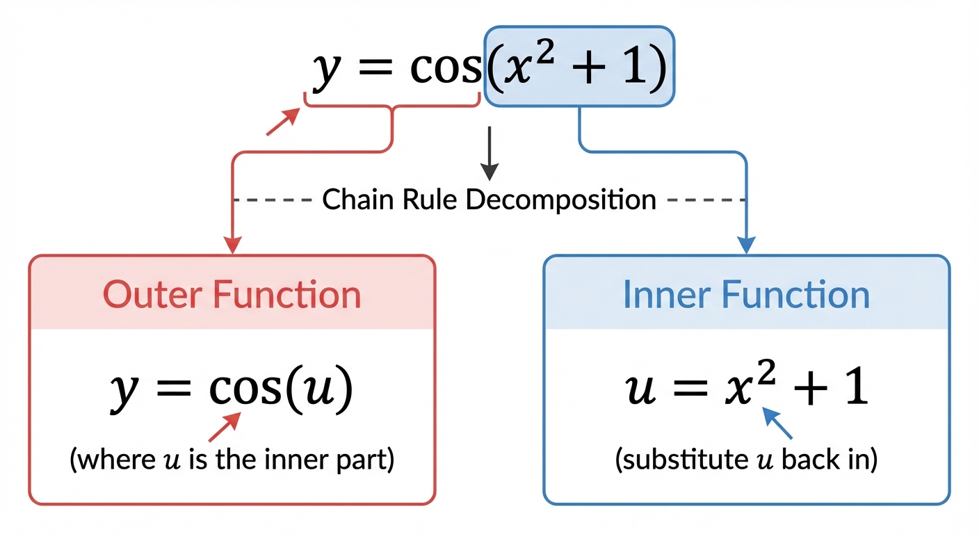
Formally, if , then its derivative is . Mastering this is non-negotiable for exam success and is a foundational concept for university-level calculus.
Worked example
Worked Example: Applying the Chain Rule to a Logarithmic Function
Let's Unpack this Composite Function 📦
Find the derivative of the function .
- 1First, we need to identify the structure of this composite function. Think 'outside-inside'. The outer function is the logarithm part, , and the inner function is the polynomial inside the brackets, .
- 2Next, we differentiate the outer function with respect to its variable, . Remember, the derivative of is .
- 3Now, we differentiate the inner function with respect to . This is a straightforward application of the power rule.
- 4Time to assemble the pieces using the chain rule formula: . We just multiply the two derivatives we found.
- 5The final, crucial step is to get our answer entirely in terms of . We substitute the original expression for back into our derivative. This gives us our final, clean answer.
Answer
3. Differentiation of Products and Quotients
Alright, let's level up our differentiation game. You've mastered the basics, but what happens when functions get complicated and start multiplying or dividing? You can't just differentiate each part separately – that's a classic exam trap! Instead, we need two powerful new tools: the Product Rule and the Quotient Rule.
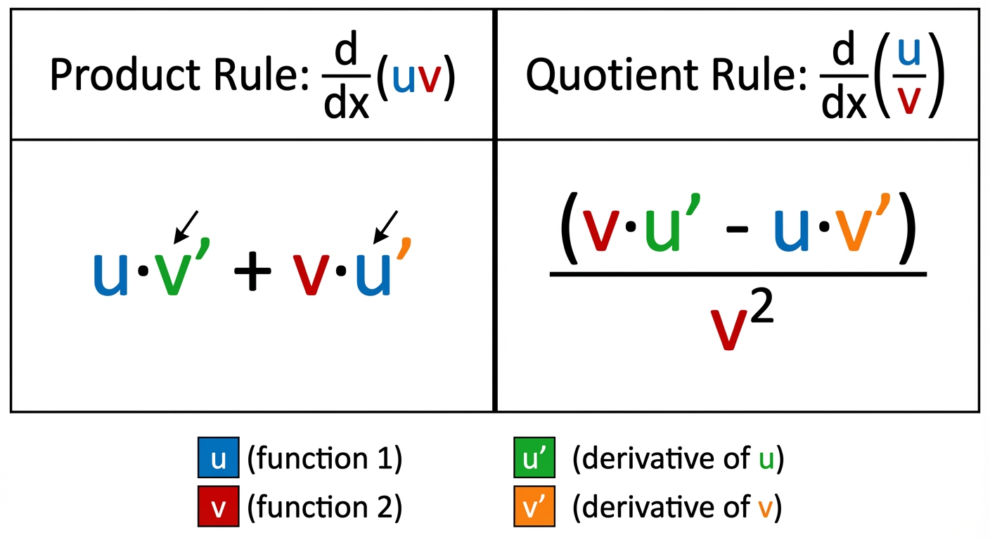
First up, the Product Rule. Use this when you have two functions multiplied together, like . Think of it as a team effort or a musical duet. Each function gets its turn to be differentiated while the other one supports it. The formula you need to memorise is: Or, in prime notation, . Since it's addition, the order doesn't strictly matter, but sticking to one form helps avoid errors.
Next, the Quotient Rule. This is for when you're dividing one function by another, like . This rule is a bit more dramatic and requires precision. The order is critical because of the subtraction. The formula is: A great way to remember this is: "low d-high, minus high d-low, square the bottom and away we go!". Mastering these isn't just about passing this exam; it's fundamental for university-level physics, engineering, and economics, where you'll model complex, interacting systems.
First up, the Product Rule. Use this when you have two functions multiplied together, like . Think of it as a team effort or a musical duet. Each function gets its turn to be differentiated while the other one supports it. The formula you need to memorise is: Or, in prime notation, . Since it's addition, the order doesn't strictly matter, but sticking to one form helps avoid errors.
Next, the Quotient Rule. This is for when you're dividing one function by another, like . This rule is a bit more dramatic and requires precision. The order is critical because of the subtraction. The formula is: A great way to remember this is: "low d-high, minus high d-low, square the bottom and away we go!". Mastering these isn't just about passing this exam; it's fundamental for university-level physics, engineering, and economics, where you'll model complex, interacting systems.
Worked example
Worked Example: Applying the Quotient Rule
Let's Tame a Beastly Fraction! 👹
Given the function , find an expression for .
- 1First, we identify our 'u' (the numerator) and 'v' (the denominator) from the fraction. This is our setup phase.
- 2Now, we differentiate both parts with respect to . Remember to use the chain rule for !
- 3Time to substitute these four components into the Quotient Rule formula: . Be meticulous with your substitution and brackets to avoid sign errors.
- 4The final, crucial step is to simplify the numerator. Look for common factors to pull out. A simplified answer is always expected and makes it easier to work with in subsequent steps (like finding stationary points).
Answer
4. Parametric and Implicit Differentiation
Alright, let's level up our differentiation game. So far, you've mostly dealt with explicit functions like , where is clearly the star of the show. But in more advanced maths, and definitely at university, relationships get more complex. Enter parametric and implicit differentiation!
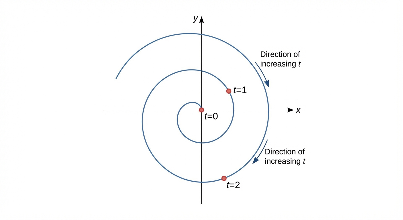
First up, parametric equations. Imagine you're tracking a drone. Instead of describing its path as in terms of , it's more natural to describe its x-position and y-position separately over time, . So you get and . Here, '' is the parameter – a third variable that controls both and . To find the gradient , we can't just differentiate with respect to directly. Instead, we use a clever application of the chain rule: Think of it as 'rate of change of y over time' divided by 'rate of change of x over time'. This is essential for physics (projectile motion) and computer graphics (creating smooth curves for animation). Once you have in terms of , finding tangents and normals is business as usual: find the gradient at a specific , find the coordinates at that , and use .
First up, parametric equations. Imagine you're tracking a drone. Instead of describing its path as in terms of , it's more natural to describe its x-position and y-position separately over time, . So you get and . Here, '' is the parameter – a third variable that controls both and . To find the gradient , we can't just differentiate with respect to directly. Instead, we use a clever application of the chain rule: Think of it as 'rate of change of y over time' divided by 'rate of change of x over time'. This is essential for physics (projectile motion) and computer graphics (creating smooth curves for animation). Once you have in terms of , finding tangents and normals is business as usual: find the gradient at a specific , find the coordinates at that , and use .
Next, implicit differentiation. This is for equations where and are all tangled up, like . It's the "it's complicated" relationship status of functions. You can't easily isolate . So, what do we do? We differentiate the entire equation with respect to , term by term. The crucial rule is: whenever you differentiate a term involving , you must multiply by . Why? Because we're assuming is secretly a function of . It's the chain rule again! For example, the derivative of with respect to is . After differentiating every term, you'll have an equation with , , and . Your final mission is to do some algebraic kung fu to isolate . This technique is a lifesaver for finding gradients on curves like circles and ellipses, and it's foundational for related rates problems you'll see in engineering and economics.
Worked example
Worked Example: Equation of a Tangent to a Parametric Curve
Let's find this tangent line's equation! 📈
A curve C is defined by the parametric equations and . Find the equation of the tangent to C at the point where .
- 1First, we need the rates of change for both x and y with respect to our parameter, t. This gives us the components for our gradient formula.
- 2Now we use the chain rule for parametric equations, , to find the gradient of the curve in terms of t.
- 3The problem asks for the tangent at a specific point, defined by . We substitute this value into our expression for to find the numerical gradient, .
- 4We have the gradient, but we need the actual coordinates of the point on the curve. We get these by substituting back into the original parametric equations.
- 5We have a point and a gradient . We can now use the point-gradient formula to find the equation of the line, usually required in the form .
Answer
Practice this in the app
Unlock the full chapter: practice questions, flashcards, mock papers and notes, free.
Continue revising