P2 Integration: The Reverse of Differentiation and Area Calculation
Let's Put the Pieces Back Together! 🧩
Introduction
1. Introduction
Alright, let's dive into one of the most fundamental concepts in A-Level Maths: Integration! Think of it as the ultimate 'undo' button for differentiation. In this chapter, we're going to explore how to reverse the process of finding gradients to instead find the area under a curve. We'll kick things off by integrating standard functions like polynomials, exponentials, and trig functions. Then, we'll level up by using our trusty trigonometric identities to simplify and solve more complex integrals. Finally, for those tricky curves that can't be integrated perfectly, we'll learn a powerful approximation technique called the Trapezium Rule. By the end of this, you'll have a solid toolkit for tackling a huge range of exam questions. Let's do this!
2. Integration of Standard Functions
Alright, let's get into it. You've mastered differentiation, which is all about finding the gradient. Integration is its inverse—like knowing the answer and having to figure out the original question. For these 'standard functions', we're essentially running our differentiation rules in reverse, but with a crucial twist: the reverse chain rule. Remember how differentiating something like would spit out a factor of 3? Well, when integrating, we have to do the opposite: divide by that coefficient of . It's the universe rebalancing itself.
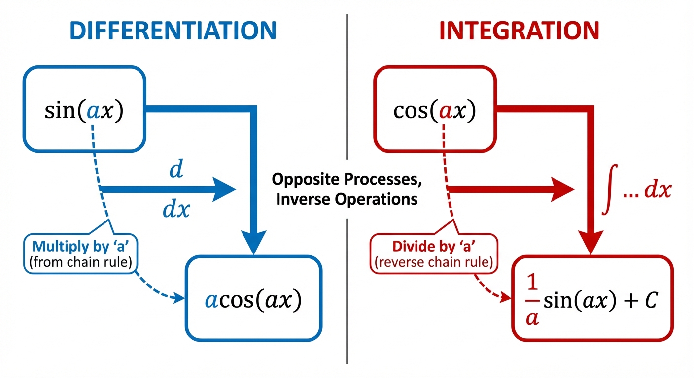
Here are your new tools, essential for exams and foundational for any STEM university course:
1. Exponentials: . This function is the MVP of modelling growth and decay, from finance to nuclear physics.
2. Reciprocals: . Notice the absolute value bars around —they are critical because you can't take the log of a negative number. Don't lose that mark!
3. Trig Functions: and . Just think of the differentiation cycle, but backwards. Super important for anything involving waves, like electrical engineering or acoustics.
4. The Special One: . This one is a direct reverse of differentiating . It looks a bit random, but it's a pattern you need to recognise instantly. And never, ever forget the '+ C' for indefinite integrals. It's the easiest point to earn... or lose. 😉
Worked example
Worked Example: Definite Integral of a Trigonometric Function
Let's Actually Solve One of These Beasts 🐲
Find the exact value of the definite integral .
- 1First, identify the core function we need to integrate. We can see the standard form , where our and . The '3' is just a constant multiplier that we can treat separately.
- 2Now, let's apply the integration rule. We integrate to get . Then, we multiply by the constant '3' that was sitting out front.
- 3Since this is a definite integral, we don't need the '+ C'. We place our result in square brackets and write the limits of integration. This sets us up to substitute the values in.
- 4Time to substitute! We plug in the upper limit () and then subtract the result of plugging in the lower limit (). Always do (upper limit) - (lower limit). Make sure your calculator is in radians!
- 5Let's simplify the expressions inside the tan functions. This is where knowing your exact trig values comes in clutch for getting that 'exact value' the question demands.
- 6Finally, substitute the known values of and to get our final answer. Job done!
Answer
3. Numerical Integration: The Trapezium Rule
Alright, so you've mastered basic integration, but what happens when you face a function that's a nightmare to integrate analytically, or maybe even impossible? Think of functions like – crucial in statistics but has no simple integral. This is where we bring in the big guns: numerical methods. The Trapezium Rule is your first major tool for approximating the value of a definite integral. The core idea is brilliantly simple: instead of finding the exact area under a curve, we chop the area into a number of vertical strips and approximate each strip as a trapezium. Why a trapezium? Because it's a much better fit for a curve than a boring old rectangle!
The formula, which is conveniently in your formula booklet (MF19), is:
Let's break that down: is the width of each trapezium strip, the '' values are the heights (or 'ordinates') at regular intervals, is the first height, and is the last. All the 'middle' heights get multiplied by 2. Simple, right?
The formula, which is conveniently in your formula booklet (MF19), is:
Let's break that down: is the width of each trapezium strip, the '' values are the heights (or 'ordinates') at regular intervals, is the first height, and is the last. All the 'middle' heights get multiplied by 2. Simple, right?
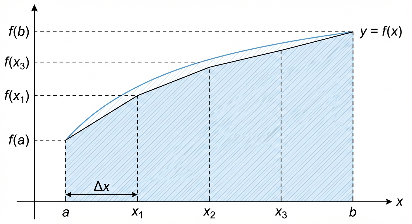
Now for the crucial exam detail: overestimate vs. underestimate. If the curve is concave up (it curves upwards, like a 'U'), the straight tops of the trapeziums will sit above the curve, giving you an overestimate. If the curve is concave down (it curves downwards, like an 'n'), the trapezium tops will sit below the curve, resulting in an underestimate. Knowing this is key for those tricky 'comment on your answer' questions. This concept is foundational for university-level engineering, physics, and data science, where you'll constantly be approximating solutions to complex problems.
Worked example
Worked Example: Applying the Trapezium Rule
Let's Calculate Some Area! 🚀
Use the trapezium rule with 4 intervals to estimate the value of giving your answer correct to 3 significant figures. State, with a reason, whether your approximation is an overestimate or an underestimate.
- 1First, we need to find the width of each trapezium, . The formula is , where and are the limits of integration and is the number of intervals.
- 2Next, we need to find the x-coordinates for each of our ordinates (the vertical lines of the trapeziums). We start at and add each time.
- 3Now, calculate the corresponding y-values (the ordinates) by substituting each x-value into the function . Pro-tip: Keep at least 4 or 5 decimal places in your working to avoid rounding errors!
- 4Time to substitute everything into the Trapezium Rule formula. Remember, it's the first y-value, plus the last y-value, plus twice the sum of all the middle ones.
- 5Calculate the final result and round to the required 3 significant figures. Don't forget this last step – easy marks to lose!
- 6Finally, we need to determine if it's an over or underestimate. Let's consider the shape of the curve . As increases, the gradient of the function also increases. This means the curve is concave up (bending upwards). Therefore, the straight tops of the trapeziums will lie above the curve.The approximation is an overestimate because the graph of is concave up.
Answer
The approximation is an overestimate because the graph of is concave up.
4. Integration Using Trigonometric Identities
Alright, so you've mastered the basic integrals, but now the game's throwing a curveball: integrating things like or . If you try to integrate these directly, you'll hit a wall. There's no standard rule for it. It's like trying to use your regular Spotify account to get exclusive pre-release tracks – it just doesn't work. You need a backstage pass, and in our case, that pass is the double angle formula for .
You probably remember this identity has a few different outfits it can wear. The ones we care about right now are and . These are our secret weapons. Why? Because we can flip them around to get the squared terms on their own.
You probably remember this identity has a few different outfits it can wear. The ones we care about right now are and . These are our secret weapons. Why? Because we can flip them around to get the squared terms on their own.
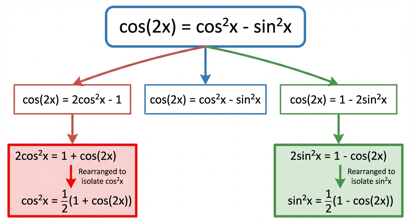
By rearranging, we get two new, super useful expressions:
1.
2.
Look at the right-hand side of these equations. We've magically turned a squared term we can't integrate into a constant and a simple cosine function that we can easily integrate. It's a total game-changer. So, whenever you see an integral with or , your first thought should be to sub in one of these identities. You're essentially swapping out a complex problem for a much simpler one. Think of it as a cheat code for integration!
Worked example
Worked Example: Integrating sin²x
Let's Solve This Thing! 🤓
Find the exact value of the definite integral .
- 1First up, we spot the problem: we can't integrate directly. This is our cue to use a trig identity. We need the one that connects to .
- 2Now, let's get by itself. A bit of algebraic shuffling gives us the expression we'll substitute into our integral.
- 3Time for the swap! We replace in the integral with our new, integration-friendly expression. Don't forget the limits of integration.
- 4Let's integrate this. We can pull the out front. The integral of is , and the integral of is (remember to divide by the derivative of the inside part!).
- 5Now we plug in our limits. Substitute the top limit () first, then subtract what you get when you substitute the bottom limit (0).
- 6Finally, simplify everything. We know that and , which makes things nice and clean. Calculate the final answer.
Answer
Practice this in the app
Unlock the full chapter: practice questions, flashcards, mock papers and notes, free.
Continue revising