Chapter S1: Representation of Data
Taming the Data Beast 📊
Introduction
1. Introduction
Welcome to S1! This is where we start turning messy lists of numbers into meaningful information. Think of yourself as a data detective. In this chapter, we're going to build your essential toolkit. First, we'll master Statistical Diagrams like histograms and box-and-whisker plots to visually represent data and spot patterns. Then, we'll dive into Measures of Central Tendency (your classic mean, median, and mode) to find the 'average' or 'typical' value in a dataset. But that's only half the story! We'll also explore Measures of Variation like standard deviation to understand how spread out or consistent the data is. Finally, we'll learn how to use coded totals such as to make tough calculations way easier. By the end of this, you'll be able to look at any dataset and tell its story. Let's get started! 💪
2. Analysis and Interpretation of Statistical Diagrams
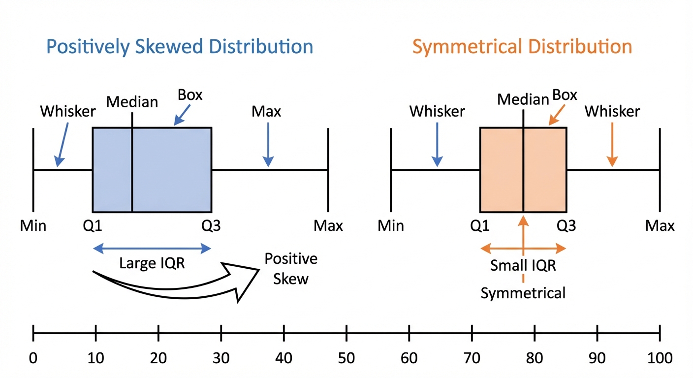
Alright, let's get visual! Raw data is like a phone book, all the info is there, but it's a nightmare to interpret. Statistical diagrams are your secret weapon to turn that chaos into clarity, and they are essential for acing S1. First up, the stem-and-leaf diagram. It's brilliant because it groups the data while keeping the original values. Super useful for seeing the shape of the distribution. For comparing two datasets, like the exam scores of two different classes, we use a back-to-back stem-and-leaf diagram. Next, we have the box-and-whisker plot, the MVP of visual comparison. It gives you a five-number summary (Min, Q1, Median, Q3, Max) in one clean graphic. You can instantly compare the median, the interquartile range (IQR, which is ), and check for skewness. This is a skill you'll use constantly in university research projects.
Now for the big one: histograms. Warning: these are NOT bar charts. Histograms are for continuous data, and the absolute key is that the area of each bar represents the frequency. This means when you have unequal class widths (which examiners love to use), you MUST plot frequency density on the y-axis. Remember this formula: Finally, we have the cumulative frequency graph (or ogive). This shows a running total. It’s perfect for estimating percentiles, like the median ( percentile) or the upper and lower quartiles ( and percentiles). This is foundational for careers in everything from finance (analysing stock returns) to medicine (studying patient recovery times). Mastering these diagrams isn't just about passing an exam; it's about learning to tell a story with data. 🚀
Worked example
Worked Example: Constructing a Histogram with Unequal Class Widths
Let's Tame Those Tricky Histograms! 🏗️
The time, (in minutes), taken by 50 students to solve a statistics problem is summarised in the table below. Draw a histogram to represent this data.
| Time ( mins) | Frequency () |
|---|---|
| 8 | |
| 15 | |
| 20 | |
| 7 |
- 1First, we check the class widths. Notice they are unequal (). This is a huge red flag that we can't just plot frequency on the y-axis. We must calculate the frequency density for each class. The formula is your best friend here.
- 2Let's calculate the class width and then the frequency density for each group. For the first group, , the class width is .
- 3Now, we repeat this for all the other classes and create a new table with our calculated values. This table is what we'll actually use to draw the histogram.
Time ( mins) 8 10 0.8 15 5 3.0 20 10 2.0 7 5 1.4 - 4Time to draw! The horizontal axis (x-axis) will be our continuous variable, 'Time ( mins)'. The vertical axis (y-axis) will be 'Frequency Density'. Make sure you choose a suitable scale for both axes.X-axis: Time (from 0 to 30)
Y-axis: Frequency Density (from 0 up to at least 3.0) - 5Finally, draw the bars. For each class, the width of the bar is the class width, and the height is the frequency density. For example, the second bar will go from to on the x-axis and have a height of . There should be no gaps between the bars. You've now created a perfect histogram!Bar 1: width 10 (0-10), height 0.8
Bar 2: width 5 (10-15), height 3.0
Bar 3: width 10 (15-25), height 2.0
Bar 4: width 5 (25-30), height 1.4
Answer
Bar 1: width 10 (0-10), height 0.8
Bar 2: width 5 (10-15), height 3.0
Bar 3: width 10 (15-25), height 2.0
Bar 4: width 5 (25-30), height 1.4
Bar 2: width 5 (10-15), height 3.0
Bar 3: width 10 (15-25), height 2.0
Bar 4: width 5 (25-30), height 1.4
3. Calculating Mean and Standard Deviation from Coded Data
Okay, let's talk about 'coded data'. Honestly, it sounds way more complicated than it is. Think of it as a 'cheat code' for dealing with large or awkward numbers. Imagine you're measuring times that are all around 120 seconds: working with instead gives small numbers that are much easier to handle. Coded data is our way of simplifying them first.
The 9709 syllabus uses a shift: the coded value is , where is a number we choose (often a value near the middle of the data). Questions give you coded totals, and , instead of and .
The 9709 syllabus uses a shift: the coded value is , where is a number we choose (often a value near the middle of the data). Questions give you coded totals, and , instead of and .
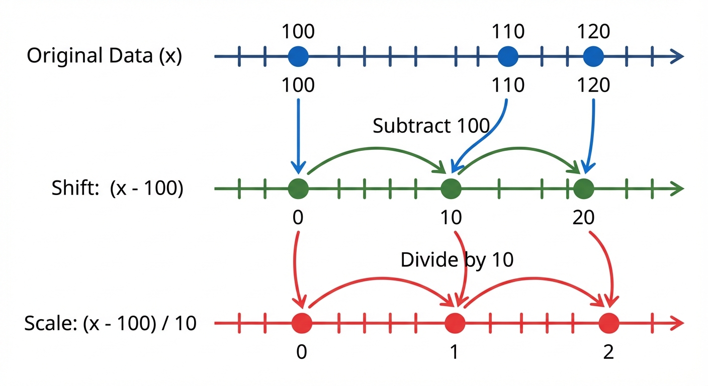
The first two lines of the picture show the shift you need: subtracting slides every value down by 100 and leaves the gaps between them unchanged. (Its third line also divides by 10; coding with a scale factor like that is not on the 9709 S1 syllabus, so you will not be asked to do it here.)
So how does this help us find the mean () and standard deviation?
• The mean slides too. The mean of is , so
• The spread does not change. Subtracting moves every value by the same amount, so the distances between them stay the same, and the standard deviation of equals the standard deviation of : Use the coded mean inside the bracket, not . If you need plain totals, .
So how does this help us find the mean () and standard deviation?
• The mean slides too. The mean of is , so
• The spread does not change. Subtracting moves every value by the same amount, so the distances between them stay the same, and the standard deviation of equals the standard deviation of : Use the coded mean inside the bracket, not . If you need plain totals, .
Worked example
Worked Example: Calculating Mean and SD from Coded Totals
Decoding the Stats 🕵️♀️
The time, seconds, taken by 20 students to complete a puzzle was recorded. The results are summarised by and . Calculate the mean and standard deviation of the time taken, .
- 1First up, let's find the mean of the coded values, . We've got their total and the number of students (), so this is a piece of cake.
- 2Now we undo the shift to find the actual mean time: add the 120 back on.
- 3Time to find the variance, using the coded totals and the coded mean.
- 4Last step! Shifting does not change the spread, so the standard deviation of is the square root of this variance, with no further adjustment.
Answer
4. Measures of Central Tendency
Alright, let's break down 'Measures of Central Tendency'. It sounds super formal, but it's just about finding the 'typical' or 'central' value in a set of data. Think of it like trying to describe your friend group with one person, who's the most representative? We have three main ways to do this:
1. The Mean (aka the Average): This is the one you probably know. You add up all the values and divide by how many values there are. The formula is . It's like finding the average amount you spend on your food delivery app each month. The mean is great, but it can be heavily skewed by outliers, those extreme values. For example, if your friend who's a pro-gamer joins your casual lobby, their crazy high score will pull the team's mean score way up.
2. The Median: This is the literal middle value when you line up all your data in order. To find its position, you use . If you have an even number of data points, you take the mean of the two middle values. The median is your MVP for data with outliers because it doesn't get affected by them. It's the true midpoint, ignoring that one friend who has 10,000 unread Snapchats when everyone else has like, 10.
3. The Mode: This one's the easiest, it's simply the value that shows up most often. If you listen to one song on repeat all day, that's the mode of your playlist. A dataset can have one mode (unimodal), two modes (bimodal), or more. It's also the only measure you can use for non-numerical data (like the most popular brand of trainers at your school).
What about Grouped Data?
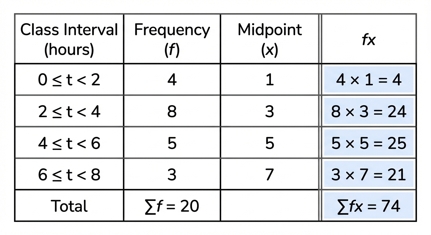
Sometimes, you don't get the raw data. Instead, you get a frequency table, like '15 students spent 0-2 hours on homework, 20 students spent 2-4 hours...'. How do you find the mean then? You can't find the exact mean, but you can calculate an Estimated Mean. To do this, you first find the midpoint of each class interval (e.g., the midpoint of 0-2 is 1). You then multiply each midpoint () by its frequency () and use the formula: . For the mode with grouped data, you just find the modal class, the group with the highest frequency. Easy!
1. The Mean (aka the Average): This is the one you probably know. You add up all the values and divide by how many values there are. The formula is . It's like finding the average amount you spend on your food delivery app each month. The mean is great, but it can be heavily skewed by outliers, those extreme values. For example, if your friend who's a pro-gamer joins your casual lobby, their crazy high score will pull the team's mean score way up.
2. The Median: This is the literal middle value when you line up all your data in order. To find its position, you use . If you have an even number of data points, you take the mean of the two middle values. The median is your MVP for data with outliers because it doesn't get affected by them. It's the true midpoint, ignoring that one friend who has 10,000 unread Snapchats when everyone else has like, 10.
3. The Mode: This one's the easiest, it's simply the value that shows up most often. If you listen to one song on repeat all day, that's the mode of your playlist. A dataset can have one mode (unimodal), two modes (bimodal), or more. It's also the only measure you can use for non-numerical data (like the most popular brand of trainers at your school).
What about Grouped Data?
Sometimes, you don't get the raw data. Instead, you get a frequency table, like '15 students spent 0-2 hours on homework, 20 students spent 2-4 hours...'. How do you find the mean then? You can't find the exact mean, but you can calculate an Estimated Mean. To do this, you first find the midpoint of each class interval (e.g., the midpoint of 0-2 is 1). You then multiply each midpoint () by its frequency () and use the formula: . For the mode with grouped data, you just find the modal class, the group with the highest frequency. Easy!
Worked example
Worked Example: Calculating the Estimated Mean from Grouped Data
Crunching the Numbers on Part-Time Job Hours 💼
The table below shows the number of hours, , worked in a week by 50 students at their part-time jobs. Estimate the mean number of hours worked.
| Hours () | ||||
|---|---|---|---|---|
| Frequency () | 12 | 20 | 13 | 5 |
- 1First up, we can't use the time intervals directly. We need a single value to represent each group, so we find the midpoint () of each class interval. To find the midpoint, just add the upper and lower bounds and divide by 2.Midpoint of is
Midpoint of is
Midpoint of is
Midpoint of is - 2Now we need to calculate the total hours worked for each group. We do this by multiplying the midpoint () by the frequency () for each row. This gives us our column. Think of it as assuming everyone in a group worked the midpoint number of hours.
- 3Next, we need the two big totals for our formula: the total number of students () and the total estimated hours worked (). Just sum up the 'frequency' and 'fx' columns.
- 4We're at the final boss! Now we just plug our totals into the formula for the estimated mean: .
- 5Don't forget the context! The question is about hours, so our final answer should be too. So, the estimated mean number of hours worked is 8.6. Also, for extra credit, which is the modal class? It's the one with the highest frequency (20 students), which is . You got this! 🙌Estimated Mean = 8.6 hours.
Answer
Estimated Mean = 8.6 hours.
5. Measures of Variation
So, we've talked about measures of central tendency like the mean and median, they give you the 'average' or 'typical' value. But that's only half the story! Imagine two friends who both average 5 hours of gaming a week. One plays for exactly 5 hours on Saturday, the other plays for 1 hour a day for 5 days and 0 on two. Same average, totally different consistency, right? That's where measures of variation (or spread) come in. They tell us how consistent or spread out the data points are.
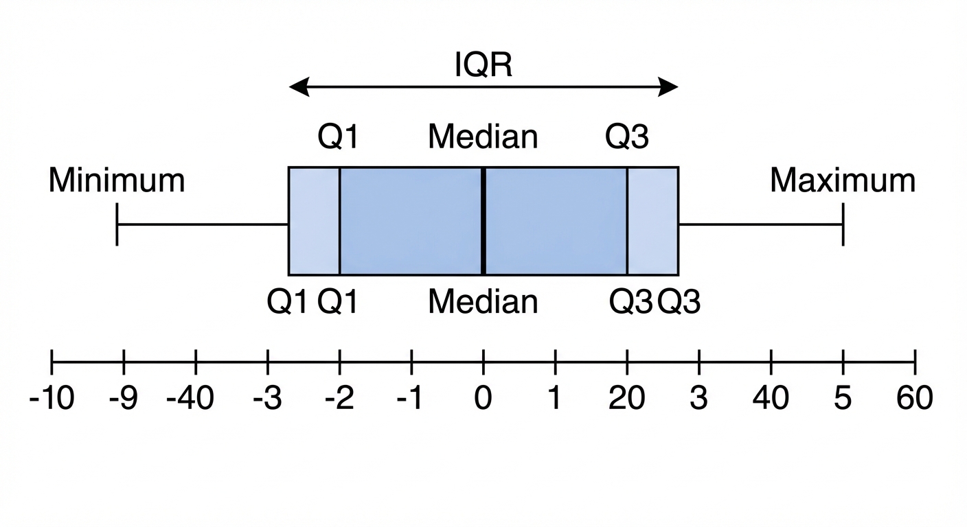
The simplest one is the range, which is just the highest value minus the lowest. It's quick, but it can be easily skewed by one crazy outlier, like that one friend who pulls an all-nighter before a new game release. A much more robust measure is the Interquartile Range (IQR). Think of it as the range of the middle 50% of your crew. We chop off the top 25% and the bottom 25% of the data and find the range of what's left. This gives a better picture of the typical spread. You find it with the formula , where is the upper quartile (75th percentile) and is the lower quartile (25th percentile).
The simplest one is the range, which is just the highest value minus the lowest. It's quick, but it can be easily skewed by one crazy outlier, like that one friend who pulls an all-nighter before a new game release. A much more robust measure is the Interquartile Range (IQR). Think of it as the range of the middle 50% of your crew. We chop off the top 25% and the bottom 25% of the data and find the range of what's left. This gives a better picture of the typical spread. You find it with the formula , where is the upper quartile (75th percentile) and is the lower quartile (25th percentile).
But the real MVP of variation is the standard deviation (represented by the Greek letter sigma, ). It measures the average distance of every data point from the mean. A small means your data points are all huddled together, super consistent, like a perfectly curated Spotify playlist. A large means your data is all over the place. To calculate it, we use the formula or the easier-to-use version . The value you get before you square root is called the variance (). Don't worry, your calculator does most of the heavy lifting here! Understanding these measures helps you see the full picture, not just the highlight reel average.
Worked example
Worked Example: Calculating Variation in Part-Time Job Hours
Let's See How Consistent These Paychecks Are 💰
The number of hours a student worked at their part-time job over 8 consecutive weeks are recorded as: 5, 8, 8, 10, 12, 15, 16, 18. Calculate the range, IQR, and the standard deviation for this data.
- 1First up, the easiest one: the range. We just find the difference between the maximum and minimum number of hours worked.
- 2Now for the IQR. We need to find the lower quartile () and upper quartile (). Since we have 8 data points, the median () is between the 4th and 5th values. is the median of the lower half (5, 8, 8, 10) and is the median of the upper half (12, 15, 16, 18).
- 3To get the standard deviation, we first need two key ingredients: the mean () and the sum of the squares (). Let's calculate those now.
- 4Finally, we plug our values for , , and into the standard deviation formula. This will tell us the average spread of weekly hours from the mean.
Answer
Practice this in the app
Unlock the full chapter: practice questions, flashcards, mock papers and notes, free.
Continue revising