S1: Discrete Random Variables
Rolling the Dice on Random Variables 🎲
Introduction
1. Introduction
Hey there! Welcome to the world of Discrete Random Variables. This might sound complicated, but it's really all about understanding the maths behind chance and probability in situations with a countable number of outcomes. Think about flipping a coin, rolling a dice, or counting the number of defective items in a batch. In this chapter, we're going to break it all down. First, we'll learn how to organize probabilities into neat Probability Distribution Tables. Then, we'll dive into calculating the Expectation (what you'd expect to happen on average) and the Variance (how spread out the results are). Finally, we'll master two super important distributions you'll see everywhere in your exams: the Binomial Distribution, for when you're running a fixed number of trials, and the Geometric Distribution, for when you're waiting for that first success. Let's get these concepts locked in so you can ace those S1 questions! 💪
2. Probability Distributions for Discrete Random Variables
Alright, let's break this down. Think of a 'discrete random variable', which we'll call , as any variable that can only take on specific, countable values. It's not continuous like height or time; it's distinct values like the score on a die (1, 2, 3, 4, 5, 6), the number of heads you get in 3 coin flips (0, 1, 2, 3), or the number of defective items in a sample. It's 'random' because we don't know which value it will take until the event happens.
So, how do we organize this information? We use a probability distribution table. This is literally just a table that lists every possible value the variable can take (we call these specific values '') and the probability of it taking that value, . It’s the ultimate summary of our random variable, showing us everything it can be and how likely each outcome is.
So, how do we organize this information? We use a probability distribution table. This is literally just a table that lists every possible value the variable can take (we call these specific values '') and the probability of it taking that value, . It’s the ultimate summary of our random variable, showing us everything it can be and how likely each outcome is.
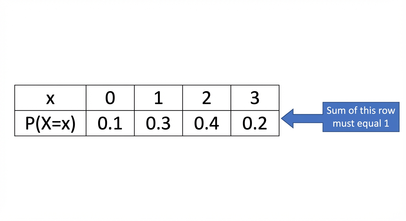
The absolute, non-negotiable, must-remember rule is this: the sum of all the probabilities in the distribution must equal 1. Seriously, tattoo this on your brain: This makes perfect sense, right? The variable has to take one of its possible values, so the total probability of all outcomes combined is 100%, or 1. Examiners love testing this, often by making you find an unknown constant in the probabilities. Mastering this table is fundamental for university-level statistics, data science, and even economics, as it's the bedrock for analysing everything from financial models to quality control in engineering.
Worked example
Worked Example: Constructing a Distribution Table and Finding an Unknown
Let's Solve for 'k' and Ace This Thing 😎
A discrete random variable can take the values 0, 1, 2, and 3. The probability distribution of is given in the table below, where is a constant.
| | 0 | 1 | 2 | 3 |
|---|---|---|---|---|
| | | | | |
(a) Find the value of .
(b) Find .
| | 0 | 1 | 2 | 3 |
|---|---|---|---|---|
| | | | | |
(a) Find the value of .
(b) Find .
- 1First things first, we need to find the value of . The golden rule for any probability distribution is that all the probabilities must add up to 1. So, we'll set up an equation by summing the probabilities in terms of .
- 2Now, let's substitute the values from the table into our equation and solve for . This is a straightforward algebra step where we combine like terms.
- 3For part (b), we need to find . This notation means 'the probability that Y is greater than or equal to 1, but less than 3'. Looking at the possible integer values for , this includes and . We don't include because the inequality is strict ().
- 4Finally, we substitute the expressions for these probabilities in terms of , and then plug in the value of that we found in step 2 to get our final answer. It's good practice to write out the full table with the numerical probabilities to avoid mistakes.
Answer
3. Expectation and Variance of a Discrete Random Variable
Alright, let's get into Expectation and Variance. Think of Expectation, or , as the long-run average outcome of a random event. It's what you'd expect to get on average if you ran an experiment an infinite number of times, like the average score on a game you played for eternity. It's the theoretical mean, often denoted by . To calculate it, we use the formula . This just means you take each possible outcome (), multiply it by its probability (), and then add them all up. It's essentially a weighted average, where the probabilities are the weights.
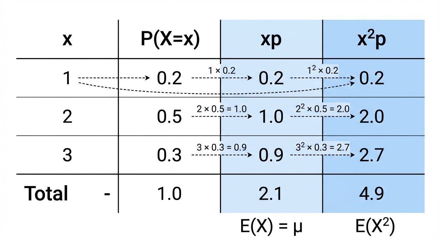
Now, Variance, or , tells us about the spread or dispersion of the outcomes. Are the results tightly clustered around the mean, or are they all over the place like your friend group's music taste? A small variance means consistency; a large variance means unpredictability. For your exams, the go-to formula is a lifesaver: . Memorise this! It translates to 'the mean of the squares minus the square of the mean'. You calculate similarly to , but you square the values before multiplying by the probability. This stuff is huge in finance for risk assessment and in scientific research for data consistency, so getting it now sets you up for uni and beyond! Remember, the standard deviation, , is just the square root of the variance, , which brings the measure of spread back into the original units. 🚀
Worked example
Worked Example: Calculating E(X) and Var(X) for a Biased Spinner
Let's Crunch Some Numbers on a Dodgy Spinner 🎲
A spinner is biased. The random variable represents the score when the spinner is spun. The probability distribution of is shown in the table below. Calculate and .
| s | 1 | 2 | 4 | 5 |
|---|---|---|---|---|
| P(S=s) | 0.4 | 0.3 | 0.2 | 0.1 |
| s | 1 | 2 | 4 | 5 |
|---|---|---|---|---|
| P(S=s) | 0.4 | 0.3 | 0.2 | 0.1 |
- 1First, let's find the expectation, . This is our expected average score. We'll use the formula by multiplying each score by its probability and summing the results.
- 2Next, we need the 'mean of the squares', which is the part of our variance formula. We square each score first, then multiply by its probability, and sum them up.
- 3Now we can calculate the variance, , using the master formula: . We just plug in the values we found in the previous steps.
- 4So, we've got our final answers. The expected mean score is 2.3, and the variance, which measures the spread of the scores, is 2.01. Job done!
Answer
4. The Binomial Distribution Model
Alright, let's level up your probability skills. The Binomial Distribution is a game-changer for a specific type of experiment, and mastering it is crucial for exams and future studies in fields like data science or engineering. Think of any situation where you have a trial that can only have two outcomes – success or failure. Did the student pass or fail? Is the product defective or not? Did the basketball player make the shot or miss? The Binomial Distribution models the number of successes, which we call , in a fixed number of independent trials.
Before you can use this powerful tool, you have to check if the situation meets four strict conditions. Think of it as a bouncer at a club – no entry unless you meet the criteria:
1. There's a fixed number of trials, which we call .
2. Each trial is independent of the others.
3. There are only two possible outcomes (success/failure).
4. The probability of success, , is constant for each trial.
Before you can use this powerful tool, you have to check if the situation meets four strict conditions. Think of it as a bouncer at a club – no entry unless you meet the criteria:
1. There's a fixed number of trials, which we call .
2. Each trial is independent of the others.
3. There are only two possible outcomes (success/failure).
4. The probability of success, , is constant for each trial.
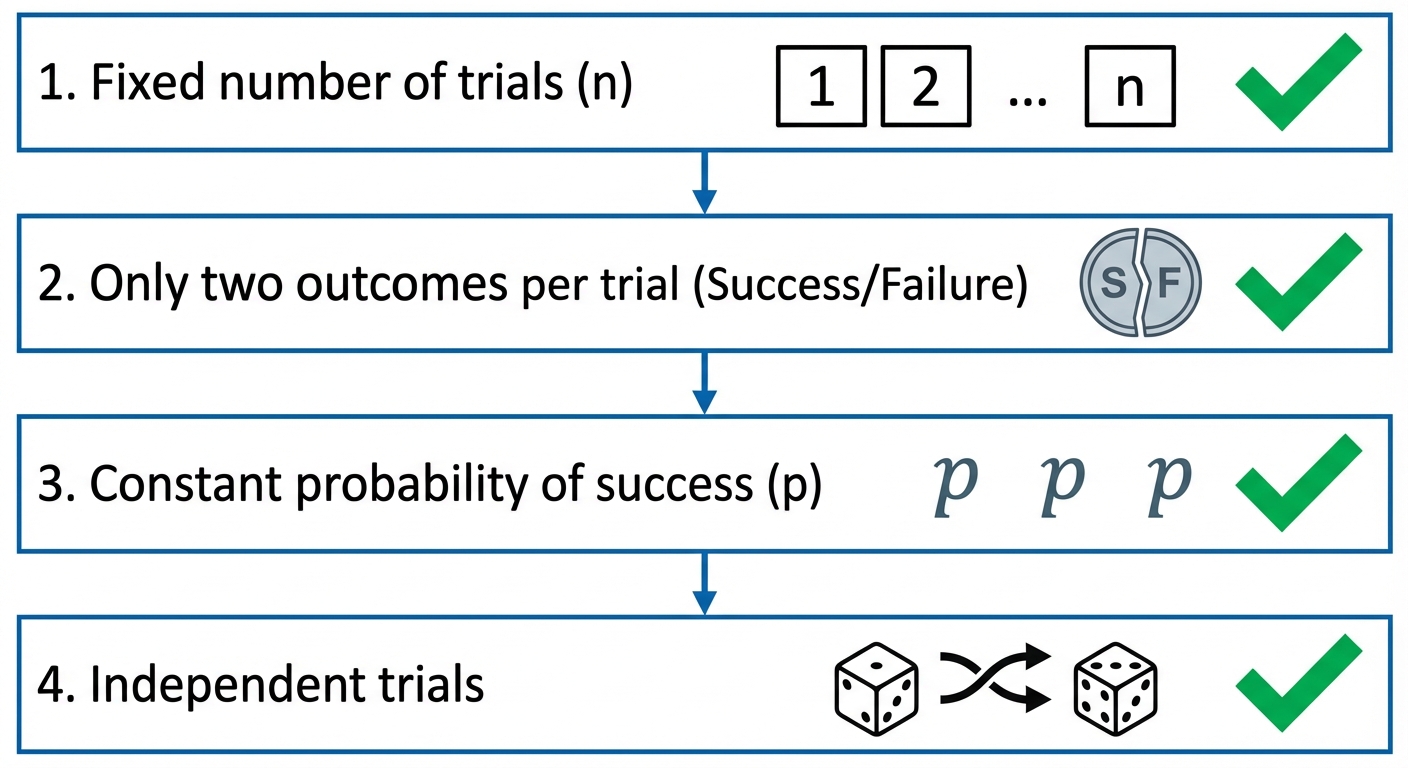
If all four conditions are met, we can say that our discrete random variable follows a Binomial Distribution, written as . The probability of getting exactly successes is given by the formula: Here, is the number of ways to choose successes from trials. It's the 'combinations' function from your calculator! The part is the probability of getting successes, and is the probability of the remaining trials being failures.
To make life even easier, there are two 'cheat code' formulas for the expectation (mean) and variance:
Expectation:
Variance:
These are incredibly useful shortcuts for exams and for understanding the 'average' outcome and the 'spread' of the results. Get these memorised – they are guaranteed marks!
Worked example
Worked Example: Manufacturing Quality Control
Are these new headphones any good? Let's find out. 🎧
A company produces wireless earbuds. It is known that 8% of the earbuds are defective. A quality control inspector randomly selects a sample of 15 earbuds. Let be the number of defective earbuds in the sample.
a) Find the probability that exactly 2 earbuds are defective.
b) Calculate the mean and variance of the number of defective earbuds in the sample.
a) Find the probability that exactly 2 earbuds are defective.
b) Calculate the mean and variance of the number of defective earbuds in the sample.
- 1First, we need to define our random variable and its distribution. We check the four conditions: fixed number of trials (), two outcomes (defective/not defective), constant probability of success (), and independence (assuming random selection). It fits! So, we can model this with a Binomial Distribution.X = \text{number of defective earbuds} \\ X \sim B(15, 0.08)
- 2For part (a), we need to find . We'll use the binomial probability formula with , , and . This means we want 2 successes (defective) and failures (not defective).P(X=x) = \binom{n}{x} p^x (1-p)^{n-x} \\ P(X=2) = \binom{15}{2} (0.08)^2 (1-0.08)^{15-2}
- 3Now, we just need to compute the values. is 105. We plug this and the other values into the calculator to get our final probability. Remember to round to an appropriate number of significant figures as per the exam instructions (usually 3 s.f.).P(X=2) = 105 \times (0.08)^2 \times (0.92)^{13} \\ P(X=2) = 105 \times 0.0064 \times 0.3430... \\ P(X=2) = 0.230 \text{ (3 s.f.)}
- 4For part (b), we calculate the mean (Expectation). This is where our shortcut formula comes in handy. It tells us the average number of defective earbuds we'd expect to find in a sample of 15.E(X) = np = 15 \times 0.08 \\ E(X) = 1.2
- 5Finally, we calculate the variance using the formula . This gives us a measure of the spread or variability in the number of defective earbuds from sample to sample.Var(X) = np(1-p) = 15 \times 0.08 \times (1-0.08) \\ Var(X) = 1.2 \times 0.92 \\ Var(X) = 1.104
Answer
Var(X) = np(1-p) = 15 \times 0.08 \times (1-0.08) \\ Var(X) = 1.2 \times 0.92 \\ Var(X) = 1.104
5. The Geometric Distribution
Alright, let's dive into the Geometric Distribution. Unlike its cousin, the Binomial distribution, where you have a fixed number of trials, the Geometric distribution is all about waiting. It models the number of trials, , required to achieve the first success. Think of it as the ultimate 'are we there yet?' of probability distributions.
For a scenario to be modelled by a Geometric distribution, it must satisfy three key conditions:
1. The trials are independent of each other.
2. Each trial has only two possible outcomes: 'success' or 'failure'.
3. The probability of success, denoted by , is constant for every trial.
If these conditions hold, we can write . The probability that your first success occurs on the -th trial is given by a beautifully simple formula: . This makes perfect sense if you break it down: you need exactly failures (each with probability ) followed by one glorious success (with probability ).
For a scenario to be modelled by a Geometric distribution, it must satisfy three key conditions:
1. The trials are independent of each other.
2. Each trial has only two possible outcomes: 'success' or 'failure'.
3. The probability of success, denoted by , is constant for every trial.
If these conditions hold, we can write . The probability that your first success occurs on the -th trial is given by a beautifully simple formula: . This makes perfect sense if you break it down: you need exactly failures (each with probability ) followed by one glorious success (with probability ).
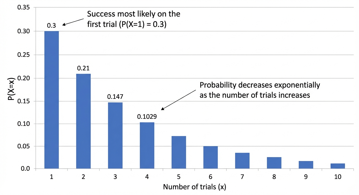
Finally, let's talk about expectation. The expected number of trials to get your first success, , is incredibly intuitive: . If your probability of hitting a target is (or 1/5), you'd intuitively expect it to take, on average, 5 attempts. This formula proves it. This concept is vital in fields like quality control (how many items to test before finding a faulty one?) and even in finance for modelling risk, so getting a solid grasp on it now will pay dividends in your university studies and beyond.
Worked example
Worked Example: Geometric Probability and Expectation
That One Elusive Shiny Pokémon ✨
A gamer is hunting for a rare 'shiny' Pokémon. The probability of encountering a shiny Pokémon in any single encounter is . The random variable is the number of encounters needed to find the first shiny Pokémon.
(a) State the distribution of .
(b) Calculate the probability that the first shiny Pokémon is found on the 500th encounter.
(c) Find the expected number of encounters needed to find the first shiny Pokémon.
(a) State the distribution of .
(b) Calculate the probability that the first shiny Pokémon is found on the 500th encounter.
(c) Find the expected number of encounters needed to find the first shiny Pokémon.
- 1First, we need to identify the distribution and its parameters. The scenario fits the geometric model because we are waiting for the first success (finding a shiny), the trials (encounters) are independent, and the probability of success is constant. So, we define our random variable .
- 2For part (b), we need to find . We use the geometric probability formula . Here, and . This means we need 499 'failures' (non-shiny encounters) followed by one 'success'.
- 3For part (c), we need to find the expected value, . This tells us the average number of encounters we'd expect to make before finding our first shiny. The formula is simply .
- 4Let's interpret the result. This means that, on average, a player should expect to have 4096 encounters to find one shiny Pokémon. It's a powerful reminder that while it could happen on the 500th try (or even the 1st!), the long-term average is defined by the probability. Good luck out there!So, the expected number of encounters is 4096.
Answer
So, the expected number of encounters is 4096.
Practice this in the app
Unlock the full chapter: practice questions, flashcards, mock papers and notes, free.
Continue revising