Chapter P2: Logarithmic and Exponential Functions
Unlocking the Secrets of Logs & Exponents 🚀
Introduction
1. Introduction
Alright, let's dive into one of the most powerful tools in your A-Level toolkit: Logarithmic and Exponential Functions! These aren't just abstract concepts; they model everything from population growth to radioactive decay. In this chapter, we're going to master three key areas. First, we'll get super comfortable with the Laws of Logarithms – they're your rules of the game for simplifying and manipulating expressions. Then, we'll apply these skills to solve tricky Exponential Equations where the unknown is stuck up in the power. Finally, we'll learn a seriously clever exam technique: Transforming to Linear Form. This is where we turn curvy, complicated graphs into nice, friendly straight lines, making them way easier to analyse. Ready to level up your algebra game? Let's get started!
2. Core Principles and Application of Logarithmic Laws
Alright, let's talk about the laws of logarithms. Honestly, these are your secret weapon for taming gnarly exponential equations. Think of them not as boring rules to memorise, but as cheat codes that let you manipulate and simplify expressions that would otherwise be a nightmare. The core idea is that logs turn multiplication into addition, division into subtraction, and powers into multiplication. It's a total game-changer.
The three fundamental laws you absolutely must know for your exams are:
1. The Product Rule:
2. The Quotient Rule:
3. The Power Rule:
Notice the beautiful symmetry with index laws? That's because logs are indices!
The three fundamental laws you absolutely must know for your exams are:
1. The Product Rule:
2. The Quotient Rule:
3. The Power Rule:
Notice the beautiful symmetry with index laws? That's because logs are indices!
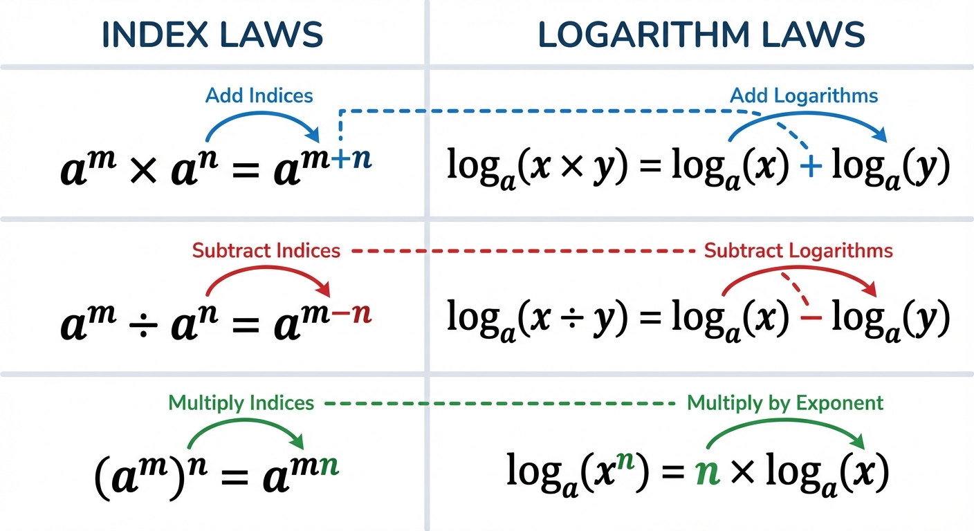
Mastering these allows you to do two key things: combine multiple log terms into a single, neat logarithm, or expand a single logarithm into multiple terms. This skill is critical not just for exam questions, but for university-level calculus and modelling in fields like finance (calculating compound interest over time) or engineering (analysing signal decay). We'll use these to simplify expressions and, in later sections, solve complex equations.
Worked example
Worked Example: Simplifying Logarithmic Expressions
Let's Combine 'Em! 💪
Express as a single logarithm.
- 1First up, we need to deal with the coefficients in front of the log terms. We'll use the power rule, , to move these coefficients 'inside' the logarithm as powers. This gets all our terms into a clean format.
- 2Now, let's simplify those powers. Remember that a power of is the same as taking the square root. This makes the numbers much easier to work with.
- 3Working from left to right, we'll combine the first two terms. Since they are being added, we use the product rule, , to merge them into a single log.
- 4Finally, we combine the remaining terms. This time we have subtraction, so we'll use the quotient rule, . This will give us our final answer as a single logarithm.
Answer
3. Solving Exponential Equations Using Logarithms
Alright team, let's talk about one of the most powerful tools in your P2 arsenal: solving exponential equations. You'll encounter equations where the unknown variable, say , is stuck up in the exponent, like . You can't just divide by 5 or take the -th root – the variable is basically 'locked' in the power. So, how do we get it down? We use its kryptonite: logarithms. The core strategy is simple but brilliant: take logarithms of both sides of the equation. You can use any base log, but your calculator's best friends are the common logarithm (base 10, written as ) and the natural logarithm (base , written as ). Once you take logs, you can use the power law of logarithms, , to bring the exponent down to the front.
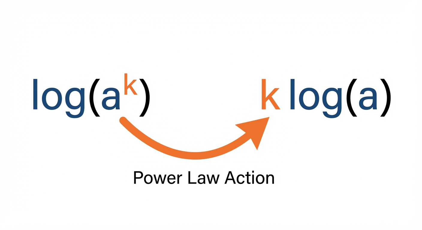
For , taking natural logs gives , which becomes . Now it's a simple linear equation: . Easy, right? This is especially slick when dealing with the number . Because and are inverse functions, they 'cancel' each other out, meaning . This shortcut is crucial for questions involving growth and decay, which are all over university science and finance courses. Mastering this isn't just about passing exams; it's fundamental for modeling real-world phenomena from population dynamics to financial investments.
Worked example
Worked Example: Solving an Equation with Base e
Let's Free that Trapped Exponent! 🕵️♂️
Solve the equation , giving your answer correct to 3 significant figures.
- 1First things first, we need to isolate the exponential term, . It's currently being multiplied by 4, so let's clear the area by dividing both sides of the equation by 4.
- 2Now that the exponential term is by itself, it's time to bring in the secret weapon. Since the base is , the natural logarithm () is the perfect tool. We'll take the natural log of both sides.
- 3Here's the magic moment. Remember that and are inverse functions, so they cancel each other out. This brings the entire exponent, , down to the main level.
- 4We've successfully beaten the hard part! Now it's just a standard two-step linear equation. To solve for , first add 1 to both sides.
- 5Finally, to get completely on its own, divide both sides by 2. Then, use your calculator to find the decimal value and round it to 3 significant figures as requested.
Answer
4. Transformation to a Linear Form
Alright, let's talk about one of the coolest tricks in a mathematician's toolkit: making curved graphs straight. Why? Because straight lines are incredibly easy to analyse. We can find their gradient and intercept with our eyes closed (well, almost!). This technique is a game-changer, turning messy exponential or power-law relationships into the simple, beautiful form of . This isn't just an exam hoop to jump through; it's a fundamental technique in fields like data science, physics, and economics, where you're constantly trying to find a model that fits experimental data. If you're heading to a STEM-based degree, this is your bread and butter.
We focus on two main types of relationships:
1. Power Law: . When you see this, think 'log-log plot'. By taking logs (base 10, , is common, but natural log, , works identically) of both sides, we get: , which simplifies using log laws to . See it? If we let and , this is literally . So, a plot of against will be a straight line where the gradient is the power, , and the Y-intercept is .
2. Exponential Law: . For this one, think 'log-linear plot'. Taking logs gives us: , which simplifies to . Now, if we let and (that's right, stays as it is!), we get . So, a plot of against will be a straight line. The gradient is , and the Y-intercept is again .
We focus on two main types of relationships:
1. Power Law: . When you see this, think 'log-log plot'. By taking logs (base 10, , is common, but natural log, , works identically) of both sides, we get: , which simplifies using log laws to . See it? If we let and , this is literally . So, a plot of against will be a straight line where the gradient is the power, , and the Y-intercept is .
2. Exponential Law: . For this one, think 'log-linear plot'. Taking logs gives us: , which simplifies to . Now, if we let and (that's right, stays as it is!), we get . So, a plot of against will be a straight line. The gradient is , and the Y-intercept is again .
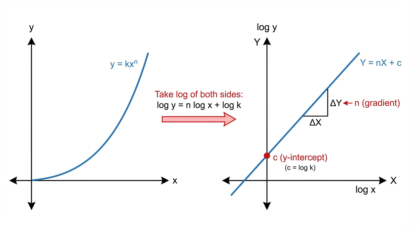
The key exam skill is to work backwards. You'll be given experimental data, plot the corresponding log graph to get a straight line, calculate its gradient and intercept, and then use those values to find the original constants (, , or ). It's like being a data detective! 🕵️
Worked example
Worked Example: Linearising Experimental Data
Let's Find Those Constants! ✨
The variables and are related by the equation , where and are constants. Experimental data for and are shown in the table below.
| | 2 | 3 | 4 | 5 | 6 |
|---|---|---|---|---|---|
| | 9.8 | 19.5 | 39.2 | 78.5 | 156.9 |
By plotting against , produce a linear graph. Use your graph to find the approximate values of and .
| | 2 | 3 | 4 | 5 | 6 |
|---|---|---|---|---|---|
| | 9.8 | 19.5 | 39.2 | 78.5 | 156.9 |
By plotting against , produce a linear graph. Use your graph to find the approximate values of and .
- 1First, we need to linearise the equation . As we saw, taking logs (base 10) of both sides is the way to go. This will tell us what to plot against what.
- 2This equation is in the form , where , , the gradient , and the Y-intercept . Our next job is to process the raw data by calculating the values of for each corresponding value.
- 3Now, we calculate the gradient of the straight-line graph. In an exam, you'd plot these points and draw a line of best fit. For here, let's just pick the first and last points from our new table to estimate the gradient, .
- 4We know that the gradient . So we can use our calculated gradient to find the value of the constant .
- 5Next, we find the Y-intercept, . We can use the straight-line equation and substitute one of our points, say , and our calculated gradient.
- 6Finally, we know that the Y-intercept . We use this to find the value of our second constant, . And that's it, we've found both constants!
Answer
Practice this in the app
Unlock the full chapter: practice questions, flashcards, mock papers and notes, free.
Continue revising