Chapter P2: Numerical Solution of Equations
Solving the Unsolvable! 🕵️♂️
Introduction
1. Introduction
Welcome to one of the most practical topics in Pure Maths! Ever wondered what happens when an equation is just too gnarly to solve exactly? We can't always find a neat answer like . That's where numerical methods come in. In this chapter, we're going to become mathematical detectives. First, we'll learn how to locate the neighbourhood of a root using the sign change rule, it's a clever trick that guarantees a root is hiding in a specific interval. Then, we'll zoom in with iterative methods, a powerful technique for getting closer and closer to the exact answer with each step. It's all about smart approximation, and it's a key skill for your exams. Let's get started!
2. Locating Roots by Change of Sign
Alright, let's get into one of the foundational ideas for solving equations numerically. Think of it like this: you're tracking your favourite streamer's subscriber count. One day they're down 100 subs (a negative change), the next they're up 500 (a positive change). To go from negative to positive, they must have passed the 'zero change' point somewhere in between, right? That's the core logic here!
In maths, a 'root' of an equation is a value of that makes . Geometrically, it's simply where the graph of crosses the x-axis. The 'change of sign' method is a super reliable way to prove that a root exists within a specific interval, say between and .
Here's the deal: If a function is continuous on an interval (meaning you can draw its graph without lifting your pen, no weird jumps or asymptotes), and the values of and have opposite signs (one is positive, the other is negative), then there must be at least one root between and .
In maths, a 'root' of an equation is a value of that makes . Geometrically, it's simply where the graph of crosses the x-axis. The 'change of sign' method is a super reliable way to prove that a root exists within a specific interval, say between and .
Here's the deal: If a function is continuous on an interval (meaning you can draw its graph without lifting your pen, no weird jumps or asymptotes), and the values of and have opposite signs (one is positive, the other is negative), then there must be at least one root between and .
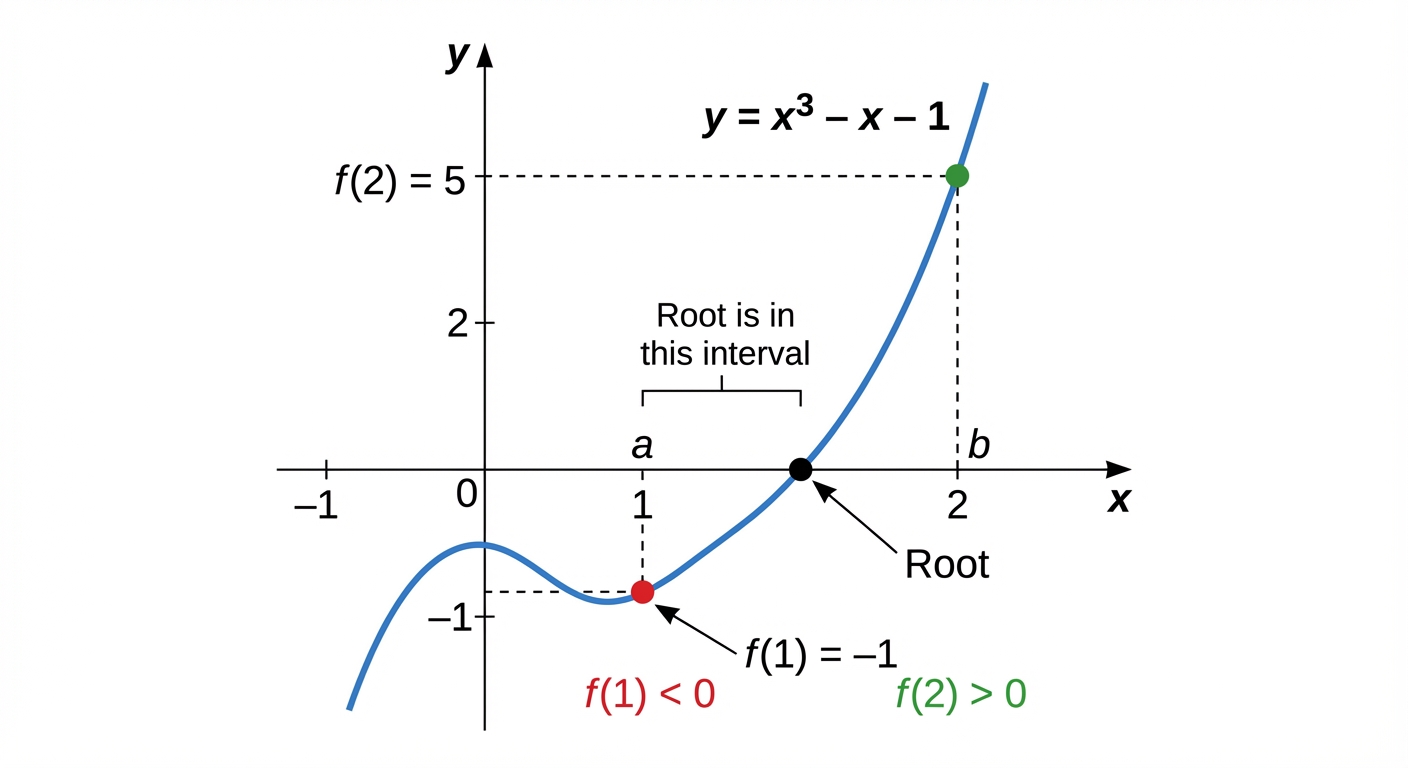
Why? Because to get from a point below the x-axis to a point above it, a continuous line has no choice but to cross it! Mathematically, we say if , a root exists in .
This concept is a classic first step in exam questions. They'll ask you to 'show a root lies in an interval' before asking you to find a more accurate approximation using methods we'll cover later. In the real world, this is fundamental for engineers finding points of equilibrium or data scientists finding optimal solutions in machine learning models. It's the starting point for zeroing in on an answer when a perfect algebraic solution isn't possible.
This concept is a classic first step in exam questions. They'll ask you to 'show a root lies in an interval' before asking you to find a more accurate approximation using methods we'll cover later. In the real world, this is fundamental for engineers finding points of equilibrium or data scientists finding optimal solutions in machine learning models. It's the starting point for zeroing in on an answer when a perfect algebraic solution isn't possible.
Worked example
Worked Example: Proving the Existence of a Root
Let's put on our detective hats and find that root! 🔍
Show that the equation has a root in the interval .
- 1First up, we need to define our function. The equation is already in the perfect form, . So, let's define and state the crucial condition for this method to work: continuity. Polynomials are continuous everywhere, so we're good to go!Let .
The function is a polynomial and is therefore continuous for all real values of . - 2Now, we test the lower bound of the interval, . We substitute this value into our function and see if the result is positive or negative.
- 3Next, we do the same for the upper bound of the interval, . We're hoping for a sign that's opposite to what we got for . Fingers crossed!
- 4This is the all-important conclusion. We've found that is negative and is positive. We must state this clearly and link it back to the continuity of the function to lock in the marks. This is the 'mic drop' moment of your proof.Since is continuous, and there is a change of sign from (negative) to (positive), there must be at least one root in the interval .
Answer
Since is continuous, and there is a change of sign from (negative) to (positive), there must be at least one root in the interval .
3. Iterative Methods for Root Approximation
Alright, so you know how some equations are just impossible to solve perfectly with regular algebra? Think of something gnarly like . There's no clean way to get 'x = ...'. This is where iterative methods come in. It's basically a 'guess and improve' strategy, like trying to find the perfect sensitivity in a game. You make a guess, see how it feels, and then make a tiny adjustment until it's just right.
First, we need to rearrange our original equation, , into the form . For example, could be rearranged to or . The goal is to create an iterative formula: This formula is our 'improvement' rule. It says that our next guess () is found by plugging our current guess () into our rearranged function, .
We start with an initial guess, , which we usually find using the sign-change method you learned about earlier. Then, we just rinse and repeat: plug in to get , plug in to get , and so on. If we chose a good rearrangement, these values will get closer and closer to the actual root. This is called convergence. It's like your Spotify algorithm getting better and better at recommending absolute bangers. The values home in on the true answer.
First, we need to rearrange our original equation, , into the form . For example, could be rearranged to or . The goal is to create an iterative formula: This formula is our 'improvement' rule. It says that our next guess () is found by plugging our current guess () into our rearranged function, .
We start with an initial guess, , which we usually find using the sign-change method you learned about earlier. Then, we just rinse and repeat: plug in to get , plug in to get , and so on. If we chose a good rearrangement, these values will get closer and closer to the actual root. This is called convergence. It's like your Spotify algorithm getting better and better at recommending absolute bangers. The values home in on the true answer.
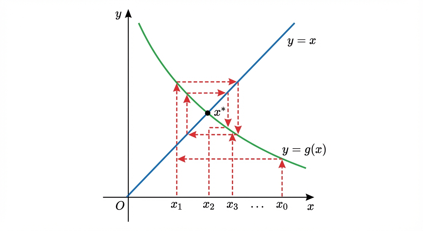
But watch out! Sometimes, the values can fly off in the opposite direction, getting further from the root with every step. That's divergence, and it means we picked a bad rearrangement. It's like trying to correct your steering when you're learning to drive and accidentally swerving even more. The final part is knowing when to stop, and this is where marks are lost. Keep full accuracy on the calculator (use ANS) and write each iterate to 2 more decimal places than the answer needs. Then look at the pattern:
• Cobweb (the values jump over and under the root): the root is trapped between consecutive iterates, so you can stop when two in a row agree to the accuracy you need.
• Staircase (the values creep steadily up or down): two iterates agreeing is not enough, because the root lies beyond both. Keep going until they agree to one more decimal place, then round. For example, from gives then , which both round to , but the root is , which is to 3 d.p.
To prove the accuracy, use a sign change: a root is to 3 d.p. if and have opposite signs. 🎉
Worked example
Worked Example: Applying an Iterative Formula
Let's Get This Root, Step-by-Step 🚀
The equation has a single real root.
a) Show that the root lies between and .
b) Use the iterative formula with a starting value of to find the root correct to 3 decimal places. Give the result of each iteration to 5 decimal places.
a) Show that the root lies between and .
b) Use the iterative formula with a starting value of to find the root correct to 3 decimal places. Give the result of each iteration to 5 decimal places.
- 1First, let's quickly do part (a) to confirm we're hunting in the right area. We define and check the sign at and .For :
For :
Since there is a change of sign from negative to positive, a root must lie between 1 and 2. Boom. - 2Now for the main event. We're given the starting value . We'll plug this into our iterative formula to get our next value, . A pro tip is to use your calculator's 'ANS' button to make this super fast.
- 3Awesome. Now we take that result for and plug it back into the formula to find . If you're using the ANS button, you just have to press the '=' key again!
- 4Let's keep the chain going, feeding the full calculator value back in each time (ANS), and writing each result to 5 decimal places.
- 5Look at the pattern: the values jump above and below each other (, , , , ...). That is a cobweb, so the root is trapped between consecutive iterates, and we may stop when two in a row agree to 3 decimal places. and both round to .
- 6Finally, prove the accuracy with a sign change on either side of , using .and , so the root lies between and : (correct to 3 d.p.)
Answer
and , so the root lies between and : (correct to 3 d.p.)
Practice this in the app
Unlock the full chapter: practice questions, flashcards, mock papers and notes, free.
Continue revising